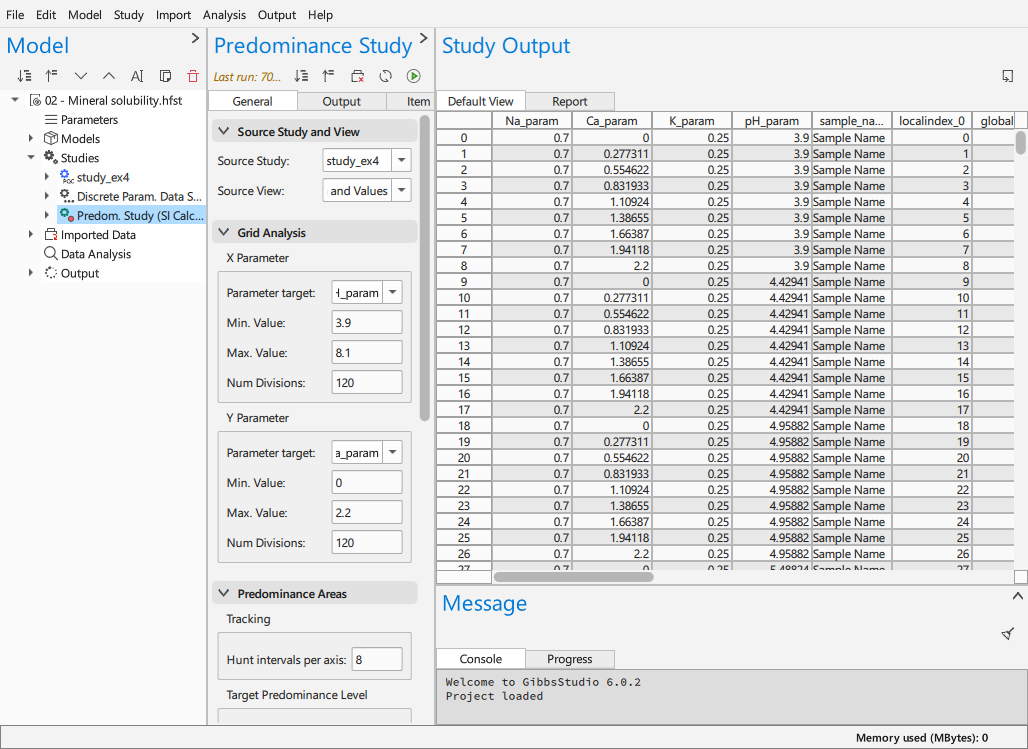
Studies
A study is what runs. Models describe, studies execute, and the results they leave behind are what Results reads.
Most study types here do not run a calculation themselves: they run another study, repeatedly, varying its parameters. That is the shape to recognise – a PHREEQC study at the bottom doing the chemistry, and a parametric, grid, discrete-data or Monte Carlo study above it deciding what to feed it. They chain, so a grid of a sweep is an ordinary thing to build.
PHREEQC Study
This entity is analogous to a PHREEQC Input. TO set it up follow the next steps:
Point it at its sources: Source Lab, Source Model, and – unless Use Model Sources is ticked, which takes them from the model – the Source Database and Source Sel.Out.
Add the PHREEQC input to solve to the Editor. It can be pasted into editor or imported through the Import file button of the Main Dock Toolbar. The PHREEQC input in GibbsStudio restricts the use of some PHREEQC Keywords, which should be removed from the input. These words are: SELECTED_OUTPUT, DATABASE, USER_GRAPH, USER_PUNCH, INCLUDE – GibbsStudio manages what each of them controls. They can be removed automatically with the Remove Not Allowed Phreeqc Sections button in the Main Dock toolbar.
Solve the Study by clicking on the Solve button in the Form Dock Toolbar.
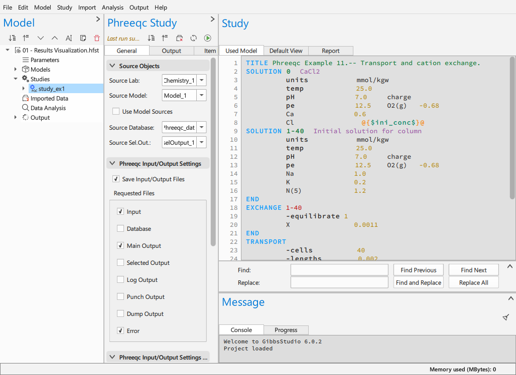
What PHREEQC writes is chosen in Phreeqc Input/Output Settings. With Save Input/Output Files ticked, Requested Files says which of PHREEQC’s own files to keep: the input, the database, the main output, the selected output, the log, the punch and dump files, and the errors. They are stored inside the project unless a Target Folder is set.
Keep what you will read. The files are written for every simulation, so a parametric study of a thousand runs writes them a thousand times, and the main output in particular is large.
To hold the project size down, the Selected Output that is kept as results can be narrowed as well: specific rows and columns can be excluded from the resulting data.
Parametric Study
Runs its target study once for every combination of the parameter values it is given. The target is usually a PHREEQC study, but it is not required to be: a parametric study of a parametric study is how a sweep gains a second dimension.
For example for a “param_1” = 1,2 and “param_2” = 1,4,5 the “Parametric Study” will run all permutations (2*3), resulting in 6 simulations.
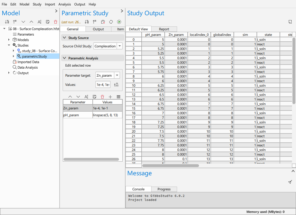
To facilitate the generation of parameter values, the following functions can be used to define them:
range(iniVal, endVal, stepSize)
linspace(iniVal, endVal, numSteps)
logspace(iniVal, endVal, numSteps, baseLog)
normal(meanVal, stdVal, numSims)
Grid Study
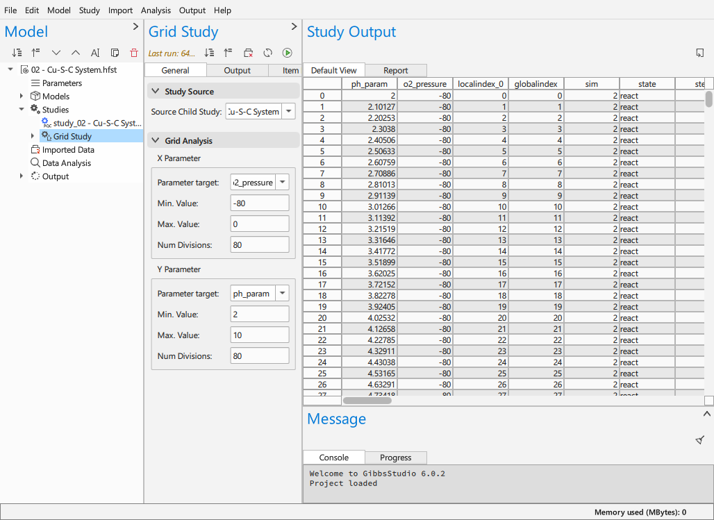
A parametric study over exactly two parameters, each on a linearly spaced range. The same result as chaining two parametric studies, set up in one place.
Function Study
Runs a function model – a set of named expressions – rather than a chemical model. It is the study to use when there is no chemistry in the problem, and it is what the “analytic” examples use to show a study type without PHREEQC in the way.
Discrete Data Study
Runs its target study once per row of a table, mapping each parameter to a column.
Where a parametric study sweeps values you choose, this takes values somebody
measured: a sampling campaign, a set of experiments, a list of cases. Point
it at an imported data set, map pH to #pH#, Ca to #Ca# and so
on, and it runs the model once for each row.
It is the third way to drive a parameterised input, alongside the parametric study above and the Monte Carlo study below – values you choose, values that were measured, values drawn from distributions. The input does not change between them.
See 03 - File as parameter input, and 03 - Saturation Indices with PHREEQC for a whole sampling campaign speciated this way.
Monte Carlo Study
A Monte Carlo Study runs another study – a PHREEQC study, or any other –
“Number of simulations” times, each time with numeric project parameters drawn
from probability distributions. It propagates the uncertainty of the inputs
(a log K, a temperature, a measured concentration) to the results. The
samples are in the study’s param table, one column per parameter; the
target’s results follow, joined by globalindex. It is part of the
Statistics module (a Professional licence).
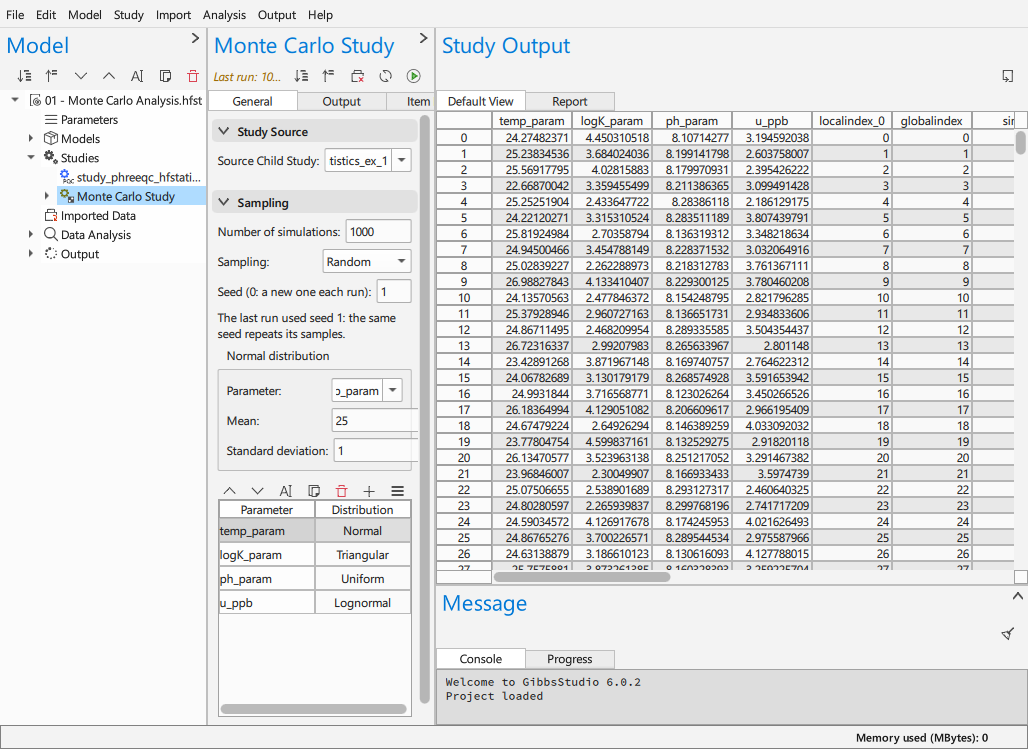
Each row of the table is a distribution of one parameter. Choosing the parameter of a new row centres the distribution on the parameter’s current value; its fields say what each value means:
Normal: mean and standard deviation.
Lognormal: the mean and standard deviation of the values themselves (not of their logarithm), e.g. 3.3 and 0.5 ppb for a concentration. Projects saved by earlier versions gave the mean and standard deviation of ln x; they are converted on opening.
Log10-normal: 10 to a normal of the given mean and standard deviation of log10 x – a log K or a log concentration drawn as K or as the concentration.
Truncated normal: a normal kept within [min, max] (no negative concentration).
Triangular: min, peak (the most likely value) and max.
Uniform: min and max (min below max; to fix a parameter, remove its distribution).
Log-uniform: every decade between min and max equally likely.
An uncertainty given as a 95% interval (the NEA-TDB’s “log K = 3.49 ± 0.2”) is about two standard deviations: std = 0.2 / 1.96. A normal log K is a lognormal K.
Sampling. Random draws each simulation independently. Latin hypercube cuts each distribution into equally probable strata, one draw in each: the same statistics from fewer runs. Each parameter is drawn independently of the others: inputs that are physically coupled (pH and the CO2 pressure) can combine into states that do not occur.
Seed. The same seed gives the same samples: a run can be repeated. New studies have seed 1; 0 draws a new seed at every run. The panel shows the seed the last run used. Each distribution has its own stream, so adding or removing one leaves the others’ draws as they were.
Simulations that fail are left out of the results (the study says how many); statistics computed from them describe the runs that succeeded.
Predominance Tracking Study
Add Track Bound. Predom. Areas Study, from the Predominance module. It generates and solves parameter combinations to track the boundaries between predominance expressions, rather than covering the whole plane: it starts coarse and spends its remaining runs where the winner changes. The predominance expressions are added by hand.
See Predominance Diagrams, and 01 - Analytic Function Predominance for what the saving amounts to against a grid study.