01 - Ion Balance and Water Types

Which samples can I trust, and what water are they? Those two questions come before any interpretation of a sampling campaign, and this example answers both from one imported file, without a single chemical calculation: the arithmetic of a water analysis is enough.

905 synthetic analyses of major ions – 25 wells, three sources, 2017 to 2020 – are imported as water samples and analysed three times, each analysis asking a narrower question than the last.

Note

The data set is synthetic. It is built to behave like a real campaign, including its bad analyses, so that the example has something to reject.

The data

source_data.tsv is read by a Chemical Sample Data Model, which is the akva plugin’s import for water analyses. It is not a general spreadsheet import: it knows what a water sample is, so it finds the columns by name – the major ions in mg/l, the electrical conductivity in µS/cm – and it is told which columns carry the sample’s point, date and category. Those three are what later lets the analyses group by well and the plots colour by source.

Three analyses of the same samples

A Cation/Anion Analysis converts the sample to meq/l and computes everything that follows from it: the ion balance, the water type, the Piper facies and the irrigation indices. All three analyses below read the same imported samples and differ only in what they keep.

All Samples keeps everything, and is how the campaign is judged. 379 of the 905 have a charge balance error within the 5 % tolerance; 526 do not, ranging from -29.8 to +36.3 % with a median of -1.4 %. By source: A 189 of 441, B 185 of 446, C only 5 of 18.

A charge balance error is not noise. The cations and anions in a water must balance, so an analysis that does not balance is missing an ion, carries a wrong unit, or has a transcription error somewhere. Source C’s analyses should be repeated; until then nothing computed from them means anything.

Balanced Samples is the same analysis with Leave unbalanced samples out set: the 379 that can be interpreted. Their water type – the ions making up at least 20 % of the total – is mostly Mg-Ca-HCO3-Cl-SO4 (130 samples) and Mg-Ca-Na-HCO3-Cl-SO4 (80). Bicarbonate waters of calcium and magnesium, some with sodium.

Median per Well adds aggregation: the balanced samples are grouped by point and reduced to their median, giving one row per well. 18 of the 25 wells have balanced samples at all. The median is deliberate – it is the statistic a single wild analysis cannot move, which is the point of aggregating in the first place. What comes out is each well’s characteristic water rather than whichever day it happened to be sampled.

The diagrams

All three plots are quick results: an analysis that knows it holds water samples can produce the diagram the discipline uses for them, already configured.

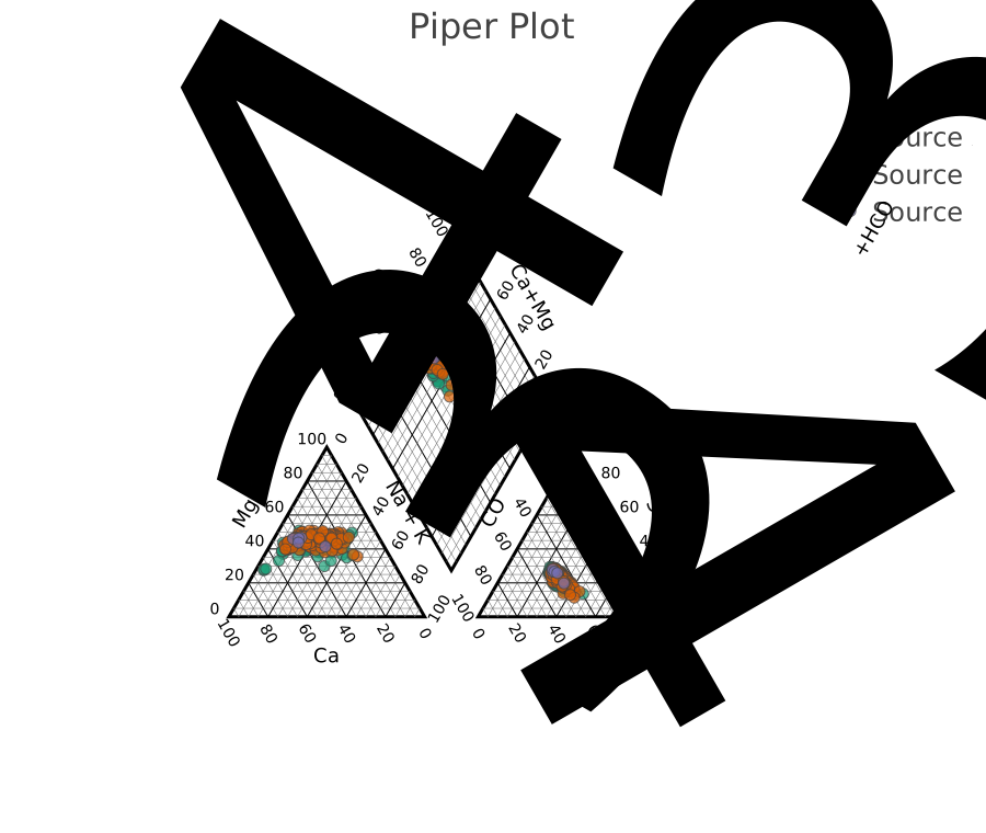
The balanced samples on a Piper diagram, coloured by source. The three sources separate more clearly in the anion triangle – chloride against sulphate – than in the cation one.

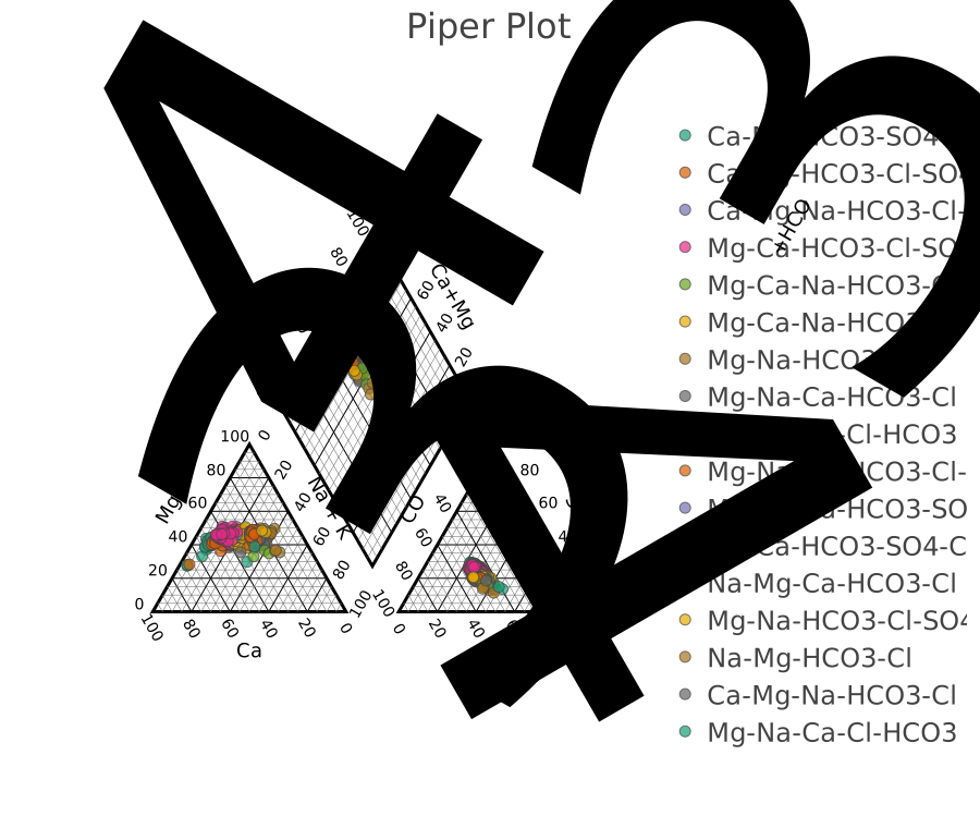
The same samples coloured by water type instead: 17 of them. Read it as a check on the classification. A type that occupies one region of the diamond is a water family; one that spreads across it is a mixture that the 20 % rule happened to name the same way.

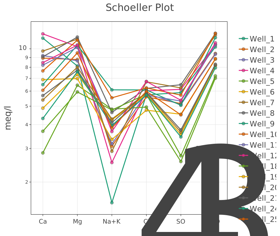
Each well’s median water on a Schoeller diagram, which plots the ions on a logarithmic scale so that proportion becomes shape. Parallel lines are waters of the same origin, one more dilute or more concentrated than the other; lines that cross are waters of different origin. This is the plot that uses Median per Well, because one line per well is readable and 379 are not.

What it concludes

379 of the 905 samples can be interpreted, and source C needs resampling. Those that remain are calcium-magnesium bicarbonate waters, some with sodium and chloride, and the Piper diagram separates the three sources by their anions.

02 - Irrigation Suitability asks what these same waters are fit for, and 03 - Saturation Indices with PHREEQC sends them to PHREEQC.

Source

The data is synthetic, but the diagrams are the standard ones of the field, implemented as they were defined:

• Piper, A. M. (1944). A graphic procedure in the geochemical interpretation of water analyses. Transactions, American Geophysical Union 25, 914-928.

• Schoeller, H. (1955). Geochimie des eaux souterraines. Revue de l’Institut Francais du Petrole 10, Paris.