02 - Principal Component Analysis

The same method as 01 - Simple Principal Component Analysis, on a real data set with four variables: Fisher’s iris measurements. 150 flowers of three species, each measured four ways – sepal length, sepal width, petal length, petal width.

It is the standard data set for this, which is the point: the result is known, so what the analysis produces can be judged rather than merely accepted.

Correlation, not covariance

This analysis works from the correlation matrix, which standardises each variable before anything else happens – it is divided by its own standard deviation, so all four arrive with a spread of one.

That is the opposite of the choice in 01 - Simple Principal Component Analysis, and the reason is that here the variables are not comparable in the way those two were. Sepal lengths vary over a wider range than petal widths, and on the covariance matrix that difference in range would decide the components by itself. Standardising asks a different and, for this data, better question: which variables vary together, regardless of how much each varies.

The rule worth carrying away: use covariance when the variables share a unit and their relative spreads are meaningful, correlation when they do not.

The result

Component	Eigenvalue	Variance	Cumulative
PC1	2.9185	72.96 %	72.96 %
PC2	0.9140	22.85 %	95.81 %
PC3	0.1468	3.67 %	99.48 %
PC4	0.0207	0.52 %	100 %

Four measurements, and two numbers carry 96 % of what they say. The loadings of the first component are 0.521, -0.269, 0.580 and 0.565: three of the four measurements pointing the same way, with sepal width the odd one out, pulling the other way and less strongly. PC1 is essentially overall size.

As in example 1, each component is signed so that its largest loading is positive.

The plots

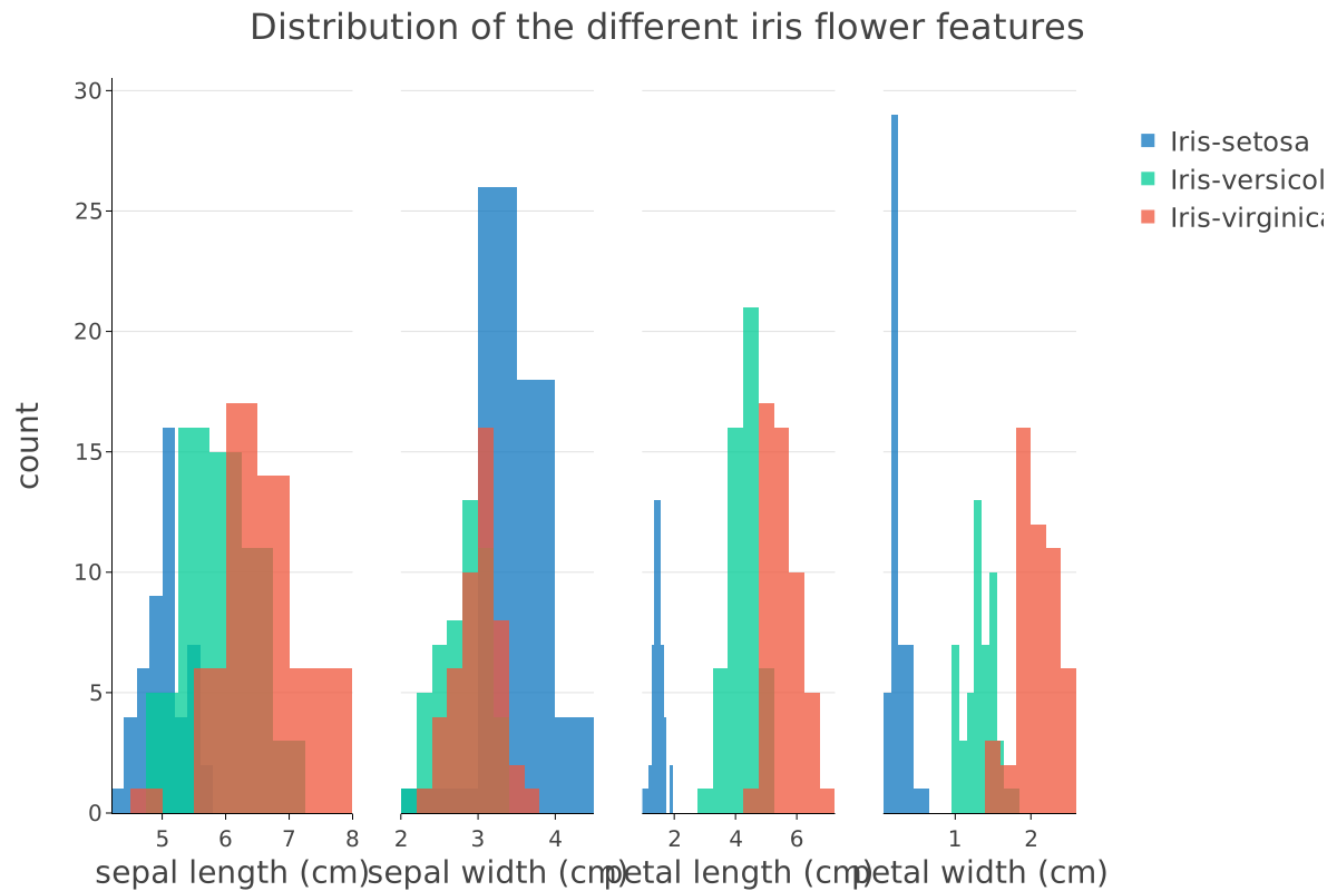
The four measurements before any analysis. Worth looking at first: the petal measurements are visibly bimodal, which is the species structure showing through, and it is what the first component will pick up.

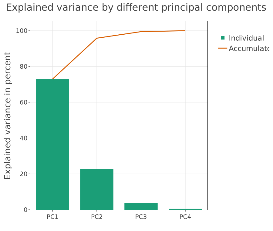
The components and how much each carries. The drop after the second is the usual justification for keeping two.

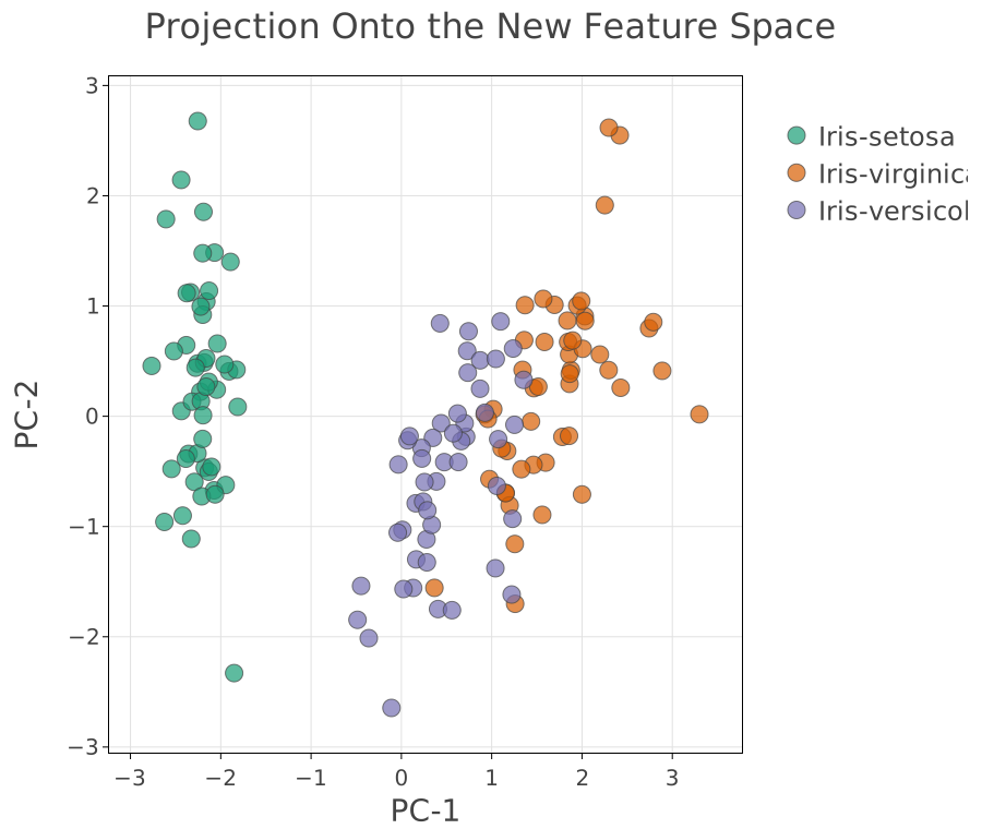
The 150 flowers on the first two components. The species separate along the first – and PCA was never told there were species. It is an unsupervised method: it found the direction of greatest variance, and in this data that direction happens to be the one that distinguishes the flowers. That is the result, and also the caution: a separation that appears in a projection is a property of the variance, and needs an explanation from outside the method before it means anything.

Checking it

The reference is R’s

prcomp(iris[, 1:4], scale. = TRUE)

which gives the same eigenvalues and the same loadings.

Other published figures for this data set differ, for two reasons worth knowing because both are easy to hit:

• The divisor. Some implementations standardise with n rather than n - 1, which makes every eigenvalue a factor n/(n - 1) larger. The structure is identical; the numbers are not.

• The file. The original iris.data in the UCI repository contains two errors against Fisher’s published table. The corrected bezdekIris file is the one used here.

Neither changes a conclusion, but both will make two correct analyses look like one wrong one.

Source

• Fisher, R. A. (1936). The use of multiple measurements in taxonomic problems. Annals of Eugenics 7(2), 179-188. The original data.

• Dua, D. and Graff, C. (2019). UCI Machine Learning Repository. University of California, Irvine, School of Information and Computer Sciences. The corrected bezdekIris file is the one read here.

• R Core Team. R: A Language and Environment for Statistical Computing. R Foundation for Statistical Computing, Vienna.