19 - Modeling Cd+2 Sorption
Cadmium sorbing to a soil, described four different ways and compared against the same measurements. Three of the four are empirical isotherms; the fourth is a mechanistic model that treats the soil as the mixture of materials it actually is.
The two figures together are the argument for doing it the harder way.
Three isotherms
TITLE Example 19.--Linear, Freundlich and Langmuir isotherms for
Cd sorption on loamy sand. Calculates Example 7.1
from Appelo and Postma, 2005. Data from Christensen, 1984.
SURFACE_MASTER_SPECIES
Linear Linear
Freundlich Freundlich
Langmuir Langmuir
SURFACE_SPECIES
Linear = Linear
Linear + Cd+2 = LinearCd+2
-log_k -100.7 # log10(0.2) - 100
-mole_balance LinearCdCl2
Freundlich = Freundlich
Freundlich + 0.722 Cd+2 = FreundlichCd+2
-log_k -102.61 # log10(0.421) + (0.722 - 1) * log10(112.4e6) - 100
-no_check
-mole_balance FreundlichCdCl2
Langmuir = Langmuir
Langmuir + Cd+2 = LangmuirCd+2
-log_k 6.56 # log10(112.4 / 30.9e-6)
-mole_balance LangmuirCdCl2
SURFACE 1
Linear 1e100 1 1
Freundlich 1e100 1 1
Langmuir 8.45e-8 1 1 # 9.5 / 112.4e6
-no_edl
SOLUTION 1
pH 6
Ca 1
Cl 2
REACTION 1
CdCl2 1
0.7e-6 in 20
PRINT
-reset false
END
Linear – sorbed is proportional to dissolved. One parameter, the distribution coefficient. No capacity limit, so it predicts unlimited sorption.
Freundlich – a power law. Two parameters, still no capacity limit, but the curvature usually fits data better.
Langmuir – a finite number of identical sites. Two parameters, and it saturates.
All three are curve fits. None refers to anything in the soil, so none can say what would happen if the pH changed, or if the organic matter were removed, or at a concentration outside the range fitted.
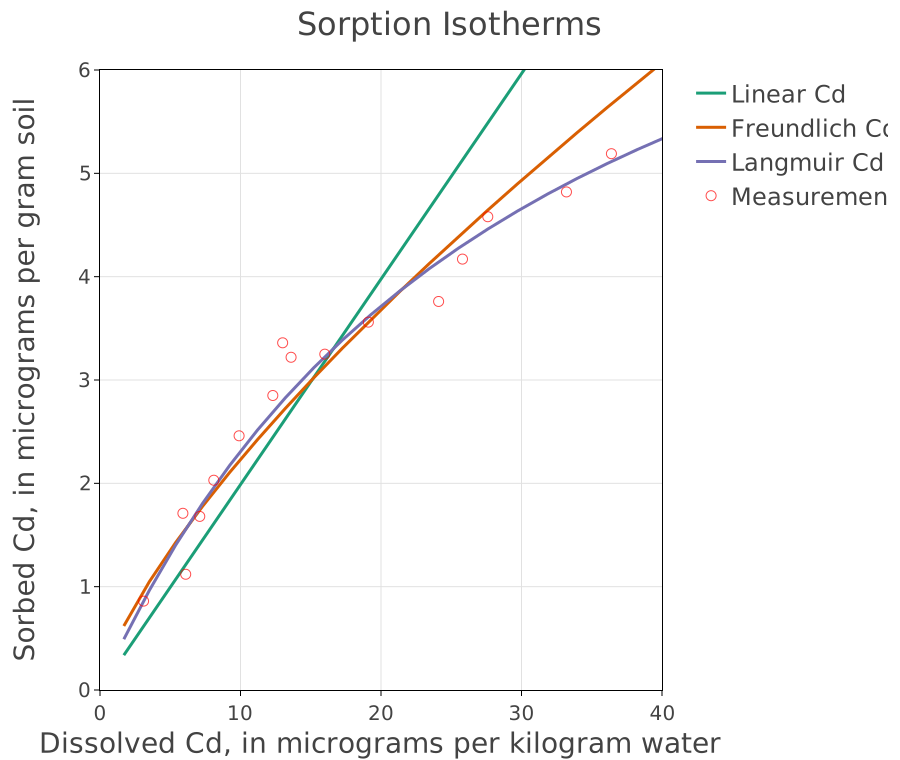
The three isotherms against the measurements. They fit – that is what fitting does – and over this range there is little to choose between them. Picking one on goodness of fit alone has no basis.
One deterministic model
TITLE Example 19B.--Cd sorption on X, Hfo and OC in loamy soil
#
PRINT
-reset false
-user_print true
SURFACE_MASTER_SPECIES
# Monodentate 60%
H_a H_aH; H_b H_bH; H_c H_cH; H_d H_dH
H_e H_eH; H_f H_fH; H_g H_gH; H_h H_hH
# Bidentate 40%
H_ab H_abH2; H_ad H_adH2; H_af H_afH2; H_ah H_ahH2
H_bc H_bcH2; H_be H_beH2; H_bg H_bgH2; H_cd H_cdH2
H_cf H_cfH2; H_ch H_chH2; H_de H_deH2; H_dg H_dgH2
SURFACE_SPECIES
H_aH = H_aH; log_k 0; H_bH = H_bH; log_k 0; H_cH = H_cH; log_k 0; \
H_dH = H_dH; log_k 0;
H_eH = H_eH; log_k 0; H_fH = H_fH; log_k 0; H_gH = H_gH; log_k 0; \
H_hH = H_hH; log_k 0;
H_abH2 = H_abH2; log_k 0; H_adH2 = H_adH2; log_k 0; H_afH2 = H_afH2; log_k 0;
H_ahH2 = H_ahH2; log_k 0; H_bcH2 = H_bcH2; log_k 0; H_beH2 = H_beH2; log_k 0;
H_bgH2 = H_bgH2; log_k 0; H_cdH2 = H_cdH2; log_k 0; H_cfH2 = H_cfH2; log_k 0;
H_chH2 = H_chH2; log_k 0; H_deH2 = H_deH2; log_k 0; H_dgH2 = H_dgH2; log_k 0;
# Protons
H_aH = H_a- + H+; log_k -1.59
H_bH = H_b- + H+; log_k -2.70
H_cH = H_c- + H+; log_k -3.82
H_dH = H_d- + H+; log_k -4.93
H_eH = H_e- + H+; log_k -6.88
H_fH = H_f- + H+; log_k -8.72
H_gH = H_g- + H+; log_k -10.56
H_hH = H_h- + H+; log_k -12.40
H_abH2 = H_abH- + H+; log_k -1.59; H_abH- = H_ab-2 + H+; log_k -2.70
H_adH2 = H_adH- + H+; log_k -1.59; H_adH- = H_ad-2 + H+; log_k -4.93
H_afH2 = H_afH- + H+; log_k -1.59; H_afH- = H_af-2 + H+; log_k -8.72
H_ahH2 = H_ahH- + H+; log_k -1.59; H_ahH- = H_ah-2 + H+; log_k -12.40
H_bcH2 = H_bcH- + H+; log_k -2.70; H_bcH- = H_bc-2 + H+; log_k -3.82
H_beH2 = H_beH- + H+; log_k -2.70; H_beH- = H_be-2 + H+; log_k -6.88
H_bgH2 = H_bgH- + H+; log_k -2.70; H_bgH- = H_bg-2 + H+; log_k -10.56
H_cdH2 = H_cdH- + H+; log_k -3.82; H_cdH- = H_cd-2 + H+; log_k -4.93
H_cfH2 = H_cfH- + H+; log_k -3.82; H_cfH- = H_cf-2 + H+; log_k -8.72
H_chH2 = H_chH- + H+; log_k -3.82; H_chH- = H_ch-2 + H+; log_k -12.40
H_deH2 = H_deH- + H+; log_k -4.93; H_deH- = H_de-2 + H+; log_k -6.88
H_dgH2 = H_dgH- + H+; log_k -4.93; H_dgH- = H_dg-2 + H+; log_k -10.56
# Calcium
H_aH + Ca+2 = H_aCa+ + H+; log_k -3.20
H_bH + Ca+2 = H_bCa+ + H+; log_k -3.20
H_cH + Ca+2 = H_cCa+ + H+; log_k -3.20
H_dH + Ca+2 = H_dCa+ + H+; log_k -3.20
H_eH + Ca+2 = H_eCa+ + H+; log_k -6.99
H_fH + Ca+2 = H_fCa+ + H+; log_k -6.99
H_gH + Ca+2 = H_gCa+ + H+; log_k -6.99
H_hH + Ca+2 = H_hCa+ + H+; log_k -6.99
H_abH2 + Ca+2 = H_abCa + 2H+; log_k -6.40
H_adH2 + Ca+2 = H_adCa + 2H+; log_k -6.40
H_afH2 + Ca+2 = H_afCa + 2H+; log_k -7.45
H_ahH2 + Ca+2 = H_ahCa + 2H+; log_k -10.2
H_bcH2 + Ca+2 = H_bcCa + 2H+; log_k -6.40
H_beH2 + Ca+2 = H_beCa + 2H+; log_k -10.2
H_bgH2 + Ca+2 = H_bgCa + 2H+; log_k -10.2
H_cdH2 + Ca+2 = H_cdCa + 2H+; log_k -6.40
H_cfH2 + Ca+2 = H_cfCa + 2H+; log_k -10.2
H_chH2 + Ca+2 = H_chCa + 2H+; log_k -10.2
H_deH2 + Ca+2 = H_deCa + 2H+; log_k -10.2
H_dgH2 + Ca+2 = H_dgCa + 2H+; log_k -10.2
# Cadmium
H_aH + Cd+2 = H_aCd+ + H+; log_k -1.52
H_bH + Cd+2 = H_bCd+ + H+; log_k -1.52
H_cH + Cd+2 = H_cCd+ + H+; log_k -1.52
H_dH + Cd+2 = H_dCd+ + H+; log_k -1.52
H_eH + Cd+2 = H_eCd+ + H+; log_k -5.57
H_fH + Cd+2 = H_fCd+ + H+; log_k -5.57
H_gH + Cd+2 = H_gCd+ + H+; log_k -5.57
H_hH + Cd+2 = H_hCd+ + H+; log_k -5.57
H_abH2 + Cd+2 = H_abCd + 2H+; log_k -3.04
H_adH2 + Cd+2 = H_adCd + 2H+; log_k -3.04
H_afH2 + Cd+2 = H_afCd + 2H+; log_k -7.09
H_ahH2 + Cd+2 = H_ahCd + 2H+; log_k -7.09
H_bcH2 + Cd+2 = H_bcCd + 2H+; log_k -3.04
H_beH2 + Cd+2 = H_beCd + 2H+; log_k -7.09
H_bgH2 + Cd+2 = H_bgCd + 2H+; log_k -7.09
H_cdH2 + Cd+2 = H_cdCd + 2H+; log_k -3.04
H_cfH2 + Cd+2 = H_cfCd + 2H+; log_k -7.09
H_chH2 + Cd+2 = H_chCd + 2H+; log_k -7.09
H_deH2 + Cd+2 = H_deCd + 2H+; log_k -7.09
H_dgH2 + Cd+2 = H_dgCd + 2H+; log_k -7.09
END
SURFACE 1
# 1 g soil = 0.7% Organic Matter ~ 3.5 mg Organic Carbon.
# 7.1 meq charge per g OC
# For Psi vs I (= ionic strength) dependence, adapt specific surface area in PHRC:
# SS = 159300 - 220800/(I)^0.09 + 91260/(I)^0.18
# Example: SS = 46514 m2/g for I = 0.003 mol/l
#
# 3.5 mg OC, 0.025 meq total charge, distributed over the sites:
# charge on 4 nHA sites: -2.84 / 4 * 3.5e-3 / 1e3 (eq)
H_a 2.48e-06 46.5e3 3.50e-03
H_b 2.48e-06; H_c 2.48e-06; H_d 2.48e-06
# charge on 4 nHB sites: 0.5 * charge on nHA sites
H_e 1.24e-06; H_f 1.24e-06; H_g 1.24e-06; H_h 1.24e-06
# charge on 12 diprotic sites: -2.84 / 12 * 3.5e-3 / 1e3
H_ab 8.28e-07; H_ad 8.28e-07; H_af 8.28e-07; H_ah 8.28e-07
H_bc 8.28e-07; H_be 8.28e-07; H_bg 8.28e-07; H_cd 8.28e-07
H_cf 8.28e-07; H_ch 8.28e-07; H_de 8.28e-07; H_dg 8.28e-07
-donnan
# 1 g soil = 2.79 mg Fe = 0.05 mmol Fe = 4.45 mg FeOOH
# 10% has ferrihydrite reactivity
Hfo_w 1e-6 600 4.45e-4
Hfo_s 0.025e-6
-equilibrate 1
EXCHANGE 1
X 55.7e-6
-equilibrate 1
SOLUTION 1
pH 6.0
Ca 1
Cl 2
Cd 1e-6
REACTION 1
CdCl2 1
2e-6 in 20
END
The fourth description abandons curve fitting. The soil is represented as what it is: humic acids, clay minerals with an exchange capacity, and hydrous ferric oxide with surface sites. Cadmium binds to each by its own chemistry, with constants measured on those materials separately – nothing is fitted to this soil’s data at all.
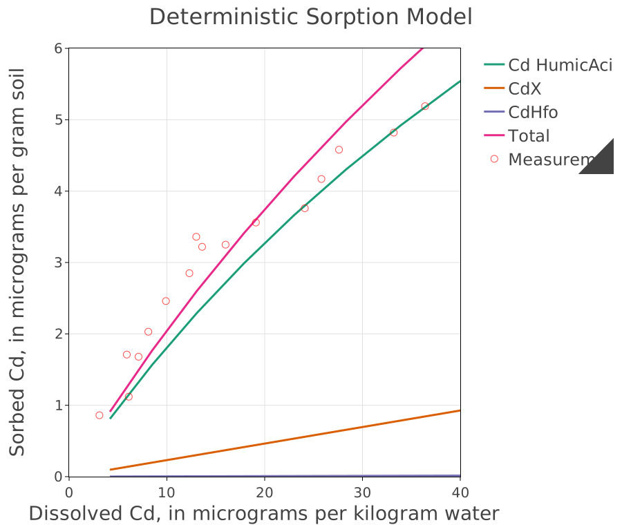
The three components and their total, against the same measurements. The total follows the data, and the individual curves say which material is responsible at each concentration – which none of the isotherms can.
That decomposition is what makes the model useful beyond the data it is drawn over. If the organic matter is what holds the cadmium, then burning it off or acidifying the soil releases it, and the model says so because it knows about humic acids. An isotherm fitted to the same points predicts nothing about any of that.
Read the two figures together as the general case for mechanistic sorption models: equivalent agreement with the data, entirely different predictive reach.
Source
Parkhurst, D. L. and Appelo, C. A. J. (2013). Description of input and examples for PHREEQC version 3. U.S. Geological Survey Techniques and Methods, book 6, chapter A43. This is Example 19 of that manual, with its measurements.
Dzombak, D. A. and Morel, F. M. M. (1990). Surface Complexation Modeling: Hydrous Ferric Oxide. Wiley, New York, for the iron oxide component.