Parameter Fitting

Running a simulation answers “given these inputs, what happens?”. Fitting answers the other question: “given what happened, what were the inputs?”

A fitting study — the Optimization module — adjusts numeric project parameters of another study until its results match data you measured. It is a least-squares fit: it minimises the sum of the squared residuals, each residual being an observed value minus the calculated one.

It is a licensed module. The study it fits can be a PHREEQC study, but it does not have to be — any study whose results depend on parameters can be fitted, including a function model.

What you need

A target study. The one being fitted, already working. Run it once by hand first: a fit of a study that does not solve is a fit of nothing.

Parameters to fit. Project Parameters the target depends on. Each one can be:

• fitted or held fixed — fix the ones you know;

• fitted on a log scale, which is right for quantities that span decades and must stay positive, a rate constant or an equilibrium constant;

• given an initial value, which is where the search starts;

• given a minimum and maximum, which the search stays inside.

Bounds are worth setting. They keep the fit inside what is physically possible — a negative concentration, a surface site density of 10⁹ — and a fit that ends up sitting on a bound is telling you something: either the bound is wrong, or the data want a value you do not believe.

Data to fit to. An imported table of observations. See Data In and Out.

A cost expression. The residual: observed minus calculated, written over the target’s view. This is the one piece people get wrong — it must be the difference, not the calculated value.

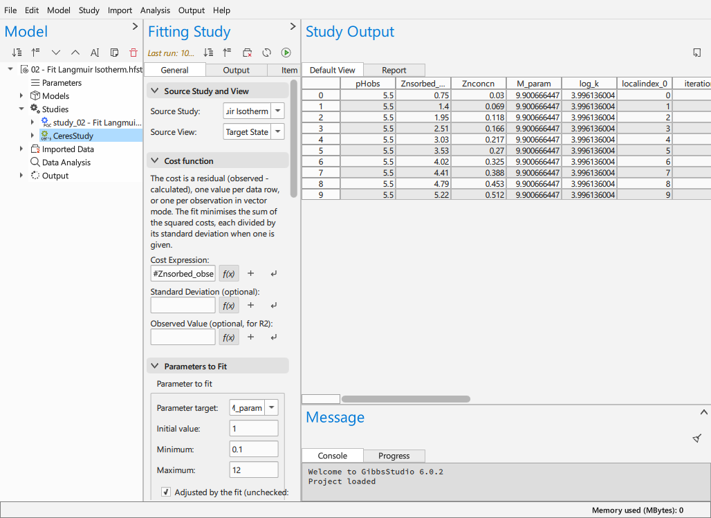
The form explains the cost in place, and shows the fitted parameters with their bounds. The Output tab beside General is where the fit’s record appears once it has run.

Scalar and vector fits

How the observations line up with the simulations decides which mode you are in.

Scalar — one residual per data row. Use this when each observation is a single number the target produces: a concentration at the end of a run, a measured total.

Vector — one residual block per target simulation, with the observations joined to the simulation’s rows by an integer index. Use this when each simulation produces a curve and you measured points along it: a titration, a kinetic experiment sampled over time.

If residuals have different reliability, weight each by its standard deviation. A measurement known to ±0.01 should not be allowed to count as much as one known to ±1.

How it searches

The fit uses Ceres’ trust-region method — Levenberg–Marquardt or dogleg — with the derivatives estimated by finite differences, which means it runs the target study many times. A fit is therefore as expensive as its target multiplied by its iterations, and that is worth a thought before fitting something slow.

A trust-region method is a local search. It finds the minimum it can reach from where it starts, not the best minimum that exists. Two consequences worth taking seriously:

• Starting values matter. Start from values that are physically sensible; if the fit runs away, that is usually what it is telling you.

• Try more than one start. If several starts converge to the same parameters, you have some reason to believe them. If they do not, the data do not determine the parameters as well as you hoped.

Reading the result

The study holds the target run at the best parameters found — so the results you plot are the fitted model — and a record of the fit itself:

The iterations

What the search did, step by step. A fit that stopped at its iteration limit has not converged, whatever the parameters say.

The parameters

Each fitted value with its standard error, its 95 % interval, and the correlations between them. Read these before believing a number. A parameter whose interval spans orders of magnitude was not determined by your data. Two parameters correlated near ±1 are not separately determined — the data constrain a combination of them, and fixing one is usually more honest than fitting both.

The statistics

SSR, s², RMSE, R², AIC. Useful for comparing fits of the same data; not evidence that a model is right.

The residuals

Worth plotting, always. Residuals should look like noise. Structure in them — drift, curvature, a run of one sign — means the model is missing something, and no amount of fitting will fix that.

Examples

• 01 – Analytic Function Fitting — the mechanics with no chemistry in the way, against the published optimum of Ceres’ own curve-fitting tutorial.

• 01 – Fit Kinetics — quartz dissolution kinetics, and the vector fit: 50 observations joined to the steps of one simulation, because a kinetic run is a single trajectory.

• 02 – Fit Langmuir Isotherm — two parameters of a sorption isotherm, and what the plateau and the initial slope each determine.

• 03 – Fit Ni Sorption — surface complexation constants from a pH edge.

• 04 – Fit Simple Titration — no fitting data at all: one residual, so a root find rather than a regression, and no statistics.