12 - Advective Diffusive Flux
Heat moving through a column alongside the solutes, and a check that the numerical method gets both right.
Where 11 - Transport and Cation Exchange verified advection against an analytical solution, this one does the same for diffusion, adds temperature as a transported quantity, and then demonstrates that the method converges at the rate it claims to.
The experiment
TITLE Example 12.--Advective and diffusive transport of heat and solutes.
Two different boundary conditions at column ends.
After diffusion temperature should equal Na-conc in mmol/l.
SOLUTION 0 24.0 mM KNO3
units mol/kgw
temp 0 # Incoming solution 0C
pH 7.0
pe 12.0 O2(g) -0.67
K 24.e-3
N(5) 24.e-3
SOLUTION 1-60 0.001 mM KCl
units mol/kgw
temp 25 # Column is at 25C
pH 7.0
pe 12.0 O2(g) -0.67
K 1e-6
Cl 1e-6
EXCHANGE_SPECIES
Na+ + X- = NaX
log_k 0.0
-gamma 4.0 0.075
H+ + X- = HX
log_k -99.
-gamma 9.0 0.0
K+ + X- = KX
log_k 0.0
gamma 3.5 0.015
EXCHANGE 1-60
KX 0.048
PRINT
-reset false
-selected_output false
-status false
TRANSPORT # Make column temperature 0C, displace Cl
-cells 60
-shifts 60
-flow_direction forward
-boundary_conditions flux flux
-lengths 0.333333
-dispersivities 0.0 # No dispersion
-diffusion_coefficient 0.0 # No diffusion
-thermal_diffusion 1.0 # No retardation for heat
END
SOLUTION 0 Fixed temp 24C, and NaCl conc (first type boundary cond) at inlet
units mol/kgw
temp 24
pH 7.0
pe 12.0 O2(g) -0.67
Na 24.e-3
Cl 24.e-3
SOLUTION 58-60 Same as soln 0 in cell 20 at closed column end (second type boundary cond)
units mol/kgw
temp 24
pH 7.0
pe 12.0 O2(g) -0.67
Na 24.e-3
Cl 24.e-3
EXCHANGE 58-60
NaX 0.048
PRINT
-selected_output true
TRANSPORT # Diffuse 24C, NaCl solution from column end
-shifts 1
-flow_direction diffusion
-boundary_conditions constant closed
-thermal_diffusion 3.0 # heat is retarded equal to Na
-diffusion_coefficient 0.3e-9 # m^2/s
-time_step 1.0e+10 # 317 years give 19 mixes
END
A column of dilute KCl at 25 °C, in equilibrium with a cation exchanger. A KNO₃ solution advects in and brings it to 0 °C. Then sodium chloride at 24 °C is allowed to diffuse in from both ends, with no heat lost through the walls – a constant-concentration boundary at one end, a closed boundary at the other.
Two boundary conditions in one column is deliberate: they are the two that occur in practice, and they produce visibly different profiles.
Heat is transported like a solute, and retarded
Temperature moves by the same advection-diffusion equation as a dissolved species, so PHREEQC transports it the same way. But heat is also stored in the solid, not only in the water, and that gives it a retardation factor exactly as sorption does for a solute.
Here the numbers line up neatly: chloride is unretarded, R = 1.0; sodium is retarded by the exchanger with R = 3.0; and the temperature is retarded by the heat capacity of the solid, also R = 3.0.
So sodium and temperature should move together, for entirely unrelated physical reasons. That coincidence is what the figure is arranged to show.
The result
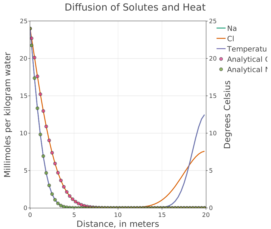
Profiles along the column, with the analytical solutions for chloride and sodium drawn over the computed ones.
Chloride has diffused furthest – nothing holds it. Sodium and temperature lag behind it by the same amount and lie on top of each other, which is the R = 3.0 they share. The asymmetry between the two ends of the column is the two boundary conditions.
The computed profiles sit on the analytical curves. That is the result: the transport is right before any chemistry is asked of it.
Second-order convergence
The example then repeats the calculation with three times as many cells. The error against the analytical solution falls by about an order of magnitude, which is what second-order accuracy predicts: refine by three, and the error should fall by roughly nine.
This is a convergence test, and it is a different and stronger check than agreeing with an analytical solution once. Agreement at one discretisation can be luck. Error falling at the predicted rate as the grid is refined says the method is doing what it claims.
For practical work the implication is the one worth carrying away: a reactive transport result is only meaningful if it is insensitive to the cell size, and the way to find out is to halve the cells and re-run.
Source
Parkhurst, D. L. and Appelo, C. A. J. (2013). Description of input and examples for PHREEQC version 3. U.S. Geological Survey Techniques and Methods, book 6, chapter A43. This is Example 12 of that manual, including the analytical solutions.