02 - Trigonometric Function Drawing

One parameter, one sweep, two curves on one plot. Where 01 - Function Surface Drawing chained studies to build a grid, this example stays in one dimension and uses the room to show two other things: a model can produce several outputs from the same inputs, and a plot can draw a trace for each of them.

The function is

\[f(x) = \sin(2 \pi x) + \cos\left(\frac{x}{2} \pi\right)\]

over \(x \in [2, 4]\).

Two outputs from one model

The Function Model defines two expressions rather than one:

f2_out = sin(2 * pi * x) + cos(x / 2 * pi)
f1_out = clamp(-1.0, sin(2 * pi * x) + cos(x / 2 * pi), +1.0)

f2_out is the function itself. f1_out is the same function with clamp holding it inside \([-1, 1]\), so wherever the original would exceed those bounds the clamped one runs flat along them. Both are computed in the same pass over the same x, and both become columns of the result table.

Note where things live. pi is a project parameter, visible everywhere; x and y belong to the model. A parameter is declared at the level that needs it, and a model carrying its own parameters is a model that can be copied into another project without dragging the rest of the project behind it.

A Function Study, xyFunction, runs the model, and a Parametric Study, xParameterRange, sweeps it:

x = range(2, 4, 0.05)

The results view is then ordered by x ascending. A plot joins its points in the order the rows arrive, so for a line plot the ordering is not cosmetic – without it the line doubles back on itself.

Reading the plot

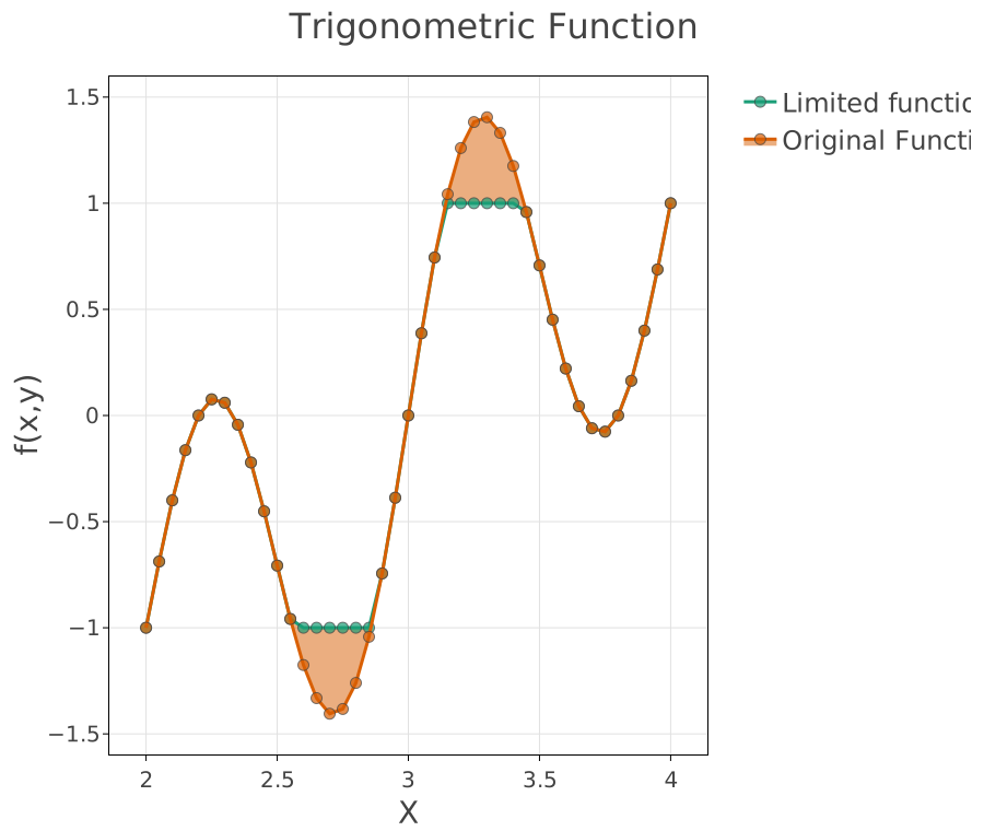
Two traces over the same sweep. Original Function is f2_out; Limited function is f1_out. They coincide everywhere the function stays within \([\pm 1]\) and separate at the peaks and troughs, where the clamped trace runs along the bound while the original carries on past it.

The shading is the Original Function trace’s area fill, set to tonexty: it fills down to the trace drawn before it rather than to zero, so the shaded band is the difference between the two – exactly what the clamp removed. Filling to the previous trace is the usual way to show a difference, a tolerance band or an envelope without computing it as a third series.

Try it

• Widen the clamp to \([-2, 2]\): the traces converge and the shaded band disappears, because the function never reaches the new bounds.

• Change pi from 3.1416 to something far from it – 2 – and recompute. Both traces change together, since both expressions read the same project parameter.

• Coarsen the sweep to range(2, 4, 0.5) to see how the sampling interval, not the function, decides how smooth a curve looks.