Results

Everything in this chapter reads results. Nothing in it runs a model.

It covers what the Analysis and Output menus add, and what lives under the Views, Data Analysis and Output branches of the project tree.

A study leaves its results in a database, and so does an import. The analytics objects – views, tables, plots and analyses – are ways of looking at what is already there. They are cheap, they can be added and deleted freely, and deleting one never costs you a calculation.

They all have the same shape:

source data  ->  a view of it  ->  a table, a plot or an analysis

The source data is a study or an imported data set. The view chooses which rows and columns of it to use. The feature on the end draws or summarises what the view produced.

Understanding the middle step is most of understanding this chapter, so it comes first.

Views

A view is a query over results: a named selection of rows and columns that behaves like a table in its own right.

Every study and every import creates default views when it computes, so there is always something to plot without building anything. Create Default Views rebuilds them.

Views matter because results are usually too big to use whole. A transport run has a row for every cell at every time step in every simulation; a plot of concentration against time needs one cell, and a profile along the column needs one time. Both are views of the same results.

The core view types are:

View	What it does
Table View	The straightforward one: a view of a results table.
Join Table View	Combines two tables on a shared index – for instance a study’s results with the parameters that produced them.
SQL Query View (Advanced)	A view you write the SQL for. The escape hatch, for anything the others cannot express.

Views chain. A view’s source can be another view, so a filter on a filter is an ordinary thing to build, and each step stays inspectable.

Filter views

A filter view is a view that keeps some rows and discards the rest. Three general ones are always available, from the view’s context menu:

Filter view	How you choose
Add Filter View by Indices	Pick a numeric field, then choose values from those actually present.
Add Filter View by String	The same for a text field.
Add Filter View using SQL	Write a SQL WHERE clause.

The first two work the same way. You name the field to filter on, and the view offers the distinct values present in the data as a list to move between available and selected. You are choosing from what is there rather than typing values and hoping, which is also why the lists have to be refreshed when the results change.

Each filter also has an active switch, so a filter can be turned off without being dismantled.

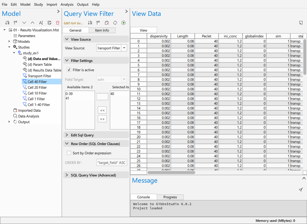
The filter above keeps cell 40 of a transport column. Its field target is soln, the available values are the cells present in the results, and below the lists are the SQL the filter builds and the row ordering – both editable when the generated query is not what you want.

With the PHREEQC plugin loaded, four presets appear for the fields a PHREEQC result always has. They are ordinary filter views with the field already set:

Preset	Field	Selects
Cell Filter View	soln	One cell, or a few, out of a transport column.
Time Filter View	step	One time step out of a run.
State Filter View	state	A kind of row – react, i_soln and so on.
Simulation Filter View	sim	One simulation out of several in an input.

The State Filter is the one that catches people out. A PHREEQC run reports more than the state you asked about: initial solutions, intermediate steps, the reacted result. Plotting without filtering on state plots all of them together, which usually looks like noise or like a line doubling back on itself.

Tables

A table presents results as columns you define. Each column has a title and an expression, so a table is not a dump of the raw fields: it is the numbers you want, in the units you want them, named as you would name them in a report.

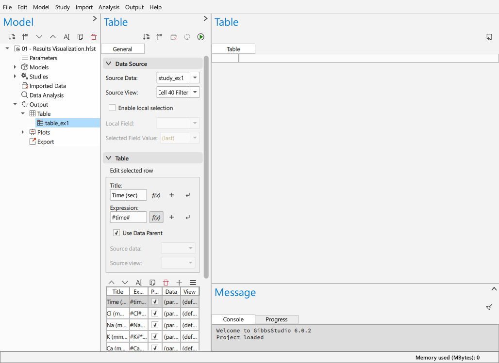
Add columns with Add Table Column, and press Compute on the form toolbar to fill the table. Linked filters update themselves; there is nothing to refresh by hand.

Add Result Table makes a table directly from a view, with a column per field, which is the quick way to look at something once.

Plots

A plot holds a layout – its axes, titles, legend and styling – and one or more traces. Each trace reads a view and draws it, so a single plot can overlay a model and the measurements it is being compared with, or two studies, or the same study filtered two ways.

Three plot presets differ only in what they set up for you:

• Add 2D Plot – an x axis and a y axis, plus a secondary y axis (y2) on the right. The secondary axis is there for the common case of two quantities with different ranges: pH against concentration, say.

• Add 3D Plot – a 3D scene.

• Add Ternary Plot – a ternary diagram, with three composition expressions a, b and c instead of x and y.

• Add Empty Plot – nothing set up, for building by hand.

Apart from the ternary plot, which takes only ternary traces, a plot is not restricted to one kind of trace. The available traces are:

Trace	Draws
Scatter	Points, lines or both. The general-purpose 2D trace, with optional area fill.
Bar	Bars, for categories.
Contour	A field over x and y as filled contours, interpolating between the points it is given.
Histogram	A distribution, binned in the browser as it draws.
2D Histogram Contour	The two-dimensional version: a density over x and y.
3D Scatter	Points or lines in a 3D scene.
3D Surface	A surface over x and y, interpolated as the contour trace is.
Ternary	A composition of three parts summing to a constant.

Plugins add their own. The predominance plugin adds a Predominance trace to the ordinary plot (see Predominance Diagrams); the water chemistry plugin brings Piper, Schoeller and USSL plots with traces of their own (see Water Chemistry); the database plugin brings a hierarchical plot with Sunburst, TreeMap and Icicle traces (see PHREEQC Databases).

Titles are expressions, like everything else, so a plot can report which slice it is showing rather than carrying a caption that goes stale:

Function Slice for y=#y#

The examples chapter is the best guide to choosing among all this. 01 - Results Visualization takes one transport result and draws it five ways – breakthrough curve, profile, colour map, surface and ternary path – and says what each one keeps and discards.

Analyses

An analysis computes something from results and leaves its own tables behind, which plots and tables can then read like any other source.

Time Series Analysis

Turns dated observations into a series that can be plotted and calculated with: it is told which columns hold the name, the date and the value, and a reference date, and it produces a time in the unit you ask for. It can also interpolate onto a regular grid, optionally conserving the total – which is what you want for a rate. Data In and Out covers it alongside the imports it usually reads.

Univariate Statistics Analysis

Statistics of one or more expressions of a study or an imported table: for each expression, the count, sum, mean, median, sample variance and standard deviation (divided by n - 1), minimum, maximum and the percentiles asked for, and a histogram. It reads the source’s view, so a Monte Carlo study’s parameters and results can be summarised directly.

• Percentiles are fractions from 0 to 1 (0.05, 0.95 for the 5th and 95th). The median and percentiles are exact: they interpolate between the sorted values as R’s quantile() (type 7) and numpy’s default do.

• Histogram: “Number of bins” equal bins between the minimum and the maximum (the last includes the maximum). Each bin has its count, its relative frequency (count / n, the field histDensity), its density (relative frequency / bin width, which can be compared with a probability density function) and its centre.

• A value that is not a number (NaN, infinity) stops the analysis, naming the expression.

The results are in stat_table (a row per expression) and histogram_table; their fields (mean_v, std_v, perc_0.05, binCentre…) can be used in plot expressions.

Note the difference from the Histogram trace: that bins the data in the browser as it draws, and the result is a picture. The analysis’s histogram is data, and can be used in tables, plots and exports.

Statistics Table

The same statistics as a results table: a row per statistic (its name, and the key of the analysis’s field), a column per expression.

Principal Component Analysis

A PCA of the expressions of a source view, on their covariance matrix or their correlation matrix (each variable standardised first). It follows R’s prcomp: variances divide by n - 1, and each component is signed so that its largest loading is positive. A constant column is left out (stat_table: analysed 0).

Choose covariance when the variables share a unit and their relative spreads are meaningful, correlation when they do not – otherwise the variable with the widest range decides the components by itself.

Its tables: eigenvalues_table (each component’s eigenvalue – the variance of its scores –, its standard deviation, and its proportion and cumulative proportion of the total variance), PC_table (the loadings, a row per variable), projected_data_table (the scores on the first “Components scored” components, with the text fields) and origin_data_table (the input).

The water chemistry plugin adds analyses of its own, for major-ion analyses and irrigation indices: see Water Chemistry.

Exports

Anything here can be written out. A plot exports as an image or as a web page that keeps its interactivity; a table exports as CSV; results export as SQL. Exports are objects in the project like the rest, so an export is repeatable rather than a thing you did once through a dialog.

Expressions

Every expression in this chapter – table columns, plot axes, plot titles, filters – uses the one language, with results fields written between hashes:

#si_Calcite# - #si_Dolomite#

Expressions is the reference for it.