04 - Fit Simple Titration¶

The odd one out, and the one that shows what a fitting study really is.

There is no data here. Nothing is being fitted to measurements. The question is: how much acid does it take to bring this water to pH 4.5? – and the answer is found by the same solver, used as a root finder.

It is PhreePlot’s simple titration example.

A fit with one residual¶

SOLUTION 1

  pH    7.05

  units mg/L

  water 0.050 kg                                           # c. 50 mL

  Na    6

  K     0.6

  Ca    124

  Mg    1.6

  Cl    11

  Alkalinity 348 as HCO3                                   # titrate this

  S(6)  3 as SO4

  Si    5.8

# could use the Fix_H+ ploy if merely wanted moles required but finding the volume needed is a bit more subtle

REACTION 1

# titrate with <titre> ml of 0.16M HCl

# 1 mL of 0.16M HCl

  HCl   0.16e-3                                            # 0.16 mM HCl

  H2O   55.56e-3

  @{$titre$}@                                                  # this@ parameter is adjusted until pH = pHwanted

END

A 50 ml sample of a calcium bicarbonate water, pH 7.05, alkalinity 348 mg/l as HCO3, is titrated with 0.16 M hydrochloric acid. The volume is the fitting parameter:

REACTION 1
  HCl   0.16e-3
  H2O   55.56e-3
  @{$titre$}@

And the residual is simply

#pH# - 4.5

Fitting data is switched off. There is one residual instead of one per row, and one unknown, so the problem is square: there is an exact answer, and the solver drives the residual to zero rather than minimising a sum of squares.

Because there is nothing to fit to, there are no statistics – no standard errors, no goodness of fit. Those quantities describe how well a model explains scattered measurements, and there are no measurements. This is worth being clear about, because the study type is the same and only the output tells you which of the two things you have done.

The general point: a Ceres Study adjusts parameters to drive an expression to zero. Fitting to data is the common use of that, not the definition of it. Anything you can write as “this quantity should equal that one” can be solved the same way – a titre, a dilution, a temperature, a mixing fraction.

Watching it converge¶

Every iteration’s PHREEQC run is kept rather than discarded, which makes the search itself inspectable.

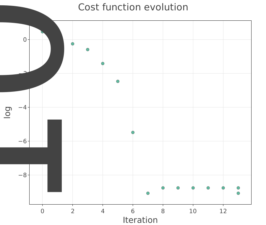
The cost function against iteration number on a logarithmic scale, falling steeply — The cost against iteration number, on a log scale. It drops steeply and then flattens at the solver’s tolerance – the shape of a well-behaved root find on a smooth problem.¶

This plot is the diagnostic to reach for when a fit misbehaves, and it is worth knowing what the failures look like. A curve that falls and then rises has stepped outside the range where the chemistry can be evaluated. One that flattens early, far above zero, has found a local minimum or has hit a parameter bound. One that descends in steps has a residual that is not smooth in the parameter – often a phase appearing and disappearing between iterations.

None of those are visible in the fitted numbers. They are visible here.

Try it¶

Ask for pH 3.0 and see how the titre and the number of iterations change.
Start titre far from the answer and watch the early iterations on the cost plot.
Replace the target with a saturation index – “add acid until calcite is at equilibrium” – which is the same problem with a different residual.

Source¶

Kinniburgh, D. G. and Cooper, D. M. (2011). PhreePlot: Creating graphical output with PHREEQC. This is PhreePlot’s simple titration example. See the PhreePlot website.
Agarwal, S., Mierle, K. and others. Ceres Solver. http://ceres-solver.org.
The thermodynamic data is wateq4f.dat, distributed with PHREEQC (Parkhurst and Appelo, 2013).