02 - Parametric Mixing

A sensitivity analysis: two waters mixed in every proportion, at a range of temperatures, and what that does to the saturation of calcite and dolomite.

03 - Mixing runs one mixing calculation. This one turns the mixing fraction into a parameter and sweeps it, which is the step from a model to a study of a model.

Parameterising the input

SOLUTION 1 

    units mol/kgw

    temp @{$temp_param$}@

    pH  8.1

    -water 1

    Ca 0.0000253

    Mg 0.0002

    C    0.0196

    Cl  6.988e-03 #charge

SAVE SOLUTION 1

END

SOLUTION 2

    units mol/kgw

    temp  @{$temp_param$}@

    pH  12.46

    -water 1

    Mg 0.2

    Ca 2.179e-02

    C   6.511e-07

    Cl  6.988e-03 #charge

SAVE SOLUTION 2

END

USE SOLUTION 1 

USE SOLUTION 2

MIX 0 

    1 @{$mix_fraction$}@

    2 @{$1-mix_fraction$}@

SAVE SOLUTION 3 

END 

The MIX block’s proportion is written as a parameter rather than a number, and so is the temperature. The input stays an ordinary PHREEQC input – the parameters are substituted before it is run – so it can still be checked by running it once with its parameters at their own values.

A Parametric Study then sweeps the two: the mixing factor from 0 to 1, and temperature over a range. Chaining the two sweeps gives the grid, exactly as in the first Core example.

The results

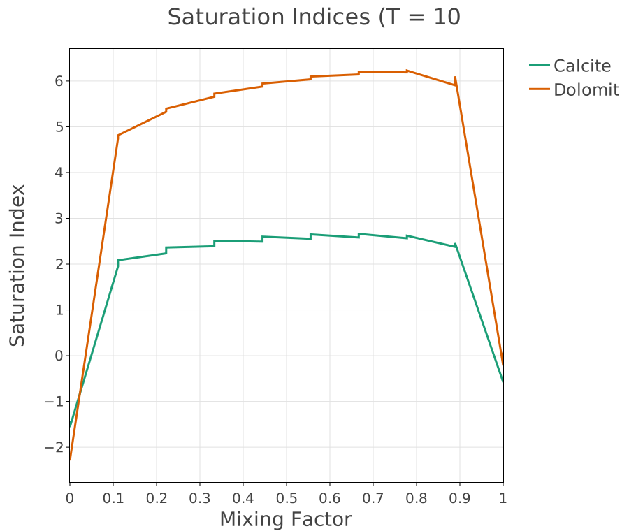
Calcite and dolomite saturation index against mixing factor at 10 °C – one slice through the grid.

Both curves dip below the straight line that would join their endpoints. That is mixing corrosion again: the two end-member waters are each at or near saturation, and intermediate mixtures are undersaturated and would dissolve carbonate. Dolomite responds more strongly than calcite, as it generally does, because its saturation index carries the product of two cation activities rather than one.

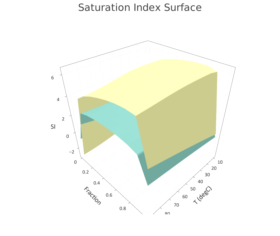
The whole grid: saturation index over mixing factor and temperature, as two surfaces. The slice above is one line across them.

Plotly draws no legend for surface traces, so read them by their relief: dolomite spans about twice the range calcite does – it reaches higher where the water is saturated and falls further where it is not, and the two cross. That is the same two-cation effect the slice shows, seen over the whole plane.

A surface is the right form for a sensitivity analysis because it answers the question the analysis is for – which input matters more. Here the gradient along the mixing axis is much the steeper of the two over this range, so the mixing proportion dominates and temperature is a second- order effect. That conclusion is visible at a glance and would take several slices to establish otherwise.

What it shows

That a parameterised input plus a parametric study turns a single calculation into a map, and that the map answers questions about sensitivity that no single run can.

Source

• Parkhurst, D. L. and Appelo, C. A. J. (2013). Description of input and examples for PHREEQC version 3. U.S. Geological Survey Techniques and Methods, book 6, chapter A43.