01 - Analytic Function Fitting
Fitting means adjusting parameters until a model agrees with measurements, and the machinery for it is the same whether the model is one line of arithmetic or a PHREEQC simulation. This example uses the one-line version, with an answer published by someone else, so the mechanism can be checked rather than believed.
It is the curve-fitting tutorial of the Ceres Solver, which is the library doing the work underneath: fit m and c of
to 67 noisy points.
The residual is the model
The thing to understand first, because everything else in this set depends on it, is what a Ceres Study is given.
It is not given a model and some data to compare. It is given an expression whose value should be zero, and it adjusts the fitting parameters until the sum of its squares is as small as it can be. Here the target is a function study with one expression:
f_out = y - exp(m*x + c)
– measured minus modelled, the residual. m and c are the fitting
parameters; x and y come from the data.
Writing the residual yourself rather than naming a model and a column is more work for a case this simple and is what makes every later case possible. A residual is just an expression, so it can weight a point, work on logarithms, combine two outputs, or compare something that was never a column – and nothing in the solver needs to know.
One residual per row
The study has fitting data – source_data.tsv, 67 rows – and for each
row it maps columns onto parameters of the same name, x and y,
evaluates the residual, and hands Ceres the result. 67 rows, 67 residuals,
two unknowns.
The fitting parameters are declared with a starting value and bounds: m
and c both start at 0.1, bounded to ±1000. The bounds are generous here
because the problem is well behaved; in the PHREEQC examples that follow they
do real work, keeping the solver away from values the chemistry cannot
evaluate.
The result
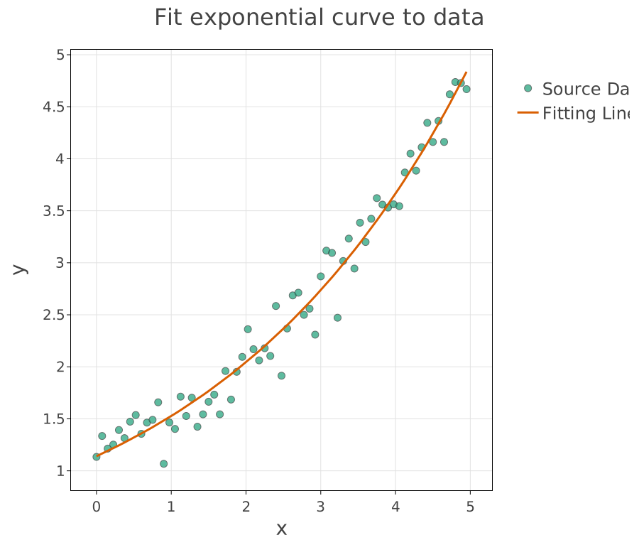
The data and the fitted curve. The fit converges to
which is the least-squares optimum Ceres publishes for this problem.
The study also reports a standard error for each parameter, in the (d) Fit Parameters output. Those are worth more attention than the fitted values. A parameter with a standard error as large as itself has not been determined by the data, however neat the curve looks – and a curve through scattered points will always look reasonable. The errors are how you tell a fit from a drawing.
Where this goes next
Everything else in this set replaces the function study with a PHREEQC study and keeps this structure exactly:
01 - Fit Kinetics fits one constant to a time series, where the residuals are joined by step rather than by row.
02 - Fit Langmuir Isotherm and 03 - Fit Ni Sorption fit two parameters each to sorption measurements.
04 - Fit Simple Titration has no data at all, and solves for a root instead.
Source
Agarwal, S., Mierle, K. and others. Ceres Solver. http://ceres-solver.org. The problem, the data and the published optimum are from the library’s curve-fitting tutorial. Ceres is the non-linear least-squares solver GibbsStudio uses.