01 - Simple Principal Component Analysis

Ten points, two variables, one answer you can check by hand. Principal component analysis is easy to apply and easy to apply wrongly, so this example runs it on a case small enough to see whole, and states the result another tool gives for the same input.

02 - Principal Component Analysis does the same on a real data set with four variables.

The data

sampledata.dat is ten pairs of x and y, strongly correlated – the classic worked example of the method. Small enough to plot as points and still recognise individual ones.

What the analysis does

A PCA Analysis is pointed at the imported table and told which columns to use, as expressions (x and y), and which matrix to work from.

Here it is the covariance matrix, which means the variables are used in their own units with their own spread. That is the right choice when the variables are commensurable – both are lengths here – and the wrong one when they are not, because a variable measured in large numbers would then dominate the result purely by its units. 02 - Principal Component Analysis makes the opposite choice, and says why.

The result is a new pair of axes: the first along the direction the data actually varies in, the second perpendicular to it. The eigenvalues say how much variance each carries:

Component	Eigenvalue	Variance
PC1	1.2840	96.3 %
PC2	0.0491	3.7 %

96.3 % on one component is what “strongly correlated” means numerically: these two variables are very nearly one variable measured twice.

A component’s sign is arbitrary – an eigenvector multiplied by -1 is the same eigenvector – so each one here is signed to make its largest loading positive. Without a rule like that, two runs of the same analysis can produce mirrored plots and look like different answers.

The plots

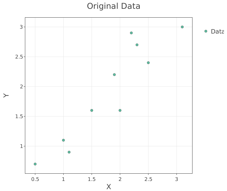
The data as measured. The elongated cloud is what PCA is about to find: there is one direction along which the points spread, and the spread across it is small.

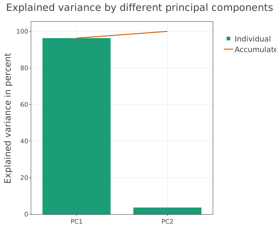
The components themselves, over the same points. The first lies along the cloud; the second is perpendicular to it, and short.

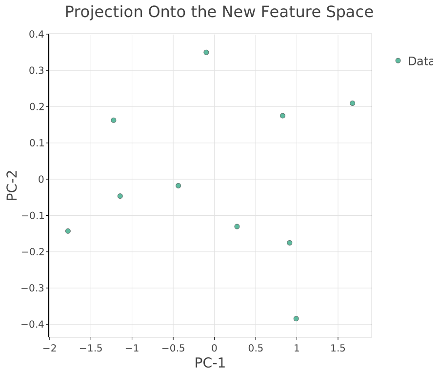
The same ten points in the new axes. This is what a PCA is for: the information has been rotated so that nearly all of it lies on one coordinate, and dropping the second would lose 3.7 % of the variance.

Checking it

The eigenvalues and loadings are those of R’s

prcomp(scale. = FALSE)

on the same data. scale. = FALSE is the covariance matrix, matching the setting used here. Running a method you can verify against a reference implementation, on data small enough to inspect, is the cheapest way to be sure you have understood what the settings mean before using them on something you cannot check.

Source

• The data set is the two-variable example used throughout the PCA literature for teaching; it is not measured data.

• R Core Team. R: A Language and Environment for Statistical Computing. R Foundation for Statistical Computing, Vienna. prcomp is R’s principal component analysis, used here as the reference.