As-O2-H2O Predominance
Arsenic speciation as a function of pH and oxygen fugacity: the diagram that says which arsenic species dominates a water, and therefore how the arsenic in it will behave. It is examples 8 and 9 of the PhreePlot manual, rebuilt here.
Arsenic is worth this treatment because its two oxidation states behave differently in almost every respect that matters – As(III) is more mobile and more toxic than As(V), and sorbs less readily to iron oxides. A diagram that shows where the boundary between them lies is a diagram about whether arsenic in an aquifer stays put.
The example also shows something diagrams of this kind usually leave out: what is second largest.
How the axes are imposed
Both axes are held at a chosen value by equilibrating with a phase, which is PhreePlot’s idiom and worth recognising because it is how most of these diagrams are built.
PHASES
Fix_H+
H+ = H+
log_k 0.0
SOLUTION 1
temp 20
units mol/kgw
As 1e-3 # total As
Na 1e-1 # background electrolyte
Cl 1e-1 charge
END
USE solution 1
EQUILIBRIUM_PHASES 1
Fix_H+ @{$-1*ph_param$}@ NaOH 10
-force_equality true
O2(g) @{$o2_pressure$}@ 0.1
END
Fix_H+ is a dummy phase – the reaction H+ = H+ with log K 0 – whose
only purpose is to be something pH can be fixed against. Equilibrating with
it at a saturation index of -pH pins the hydrogen ion activity, with NaOH
as the reagent free to enter or leave. The negation in
@{$-1*ph_param$}@ is this definition, not an adjustment: a saturation
index of -7 is pH 7.
O2(g) at a given log fugacity fixes the redox state the same way. The
solution itself is 1 mmol/l As in a 0.1 mol/l NaCl background at 20 °C, with
chloride balancing the charge.
The grid runs pH 2 to 12 and log fO2 from -90 to 0 – which is far wider than water is stable over, and deliberately so: the diagram marks where it has left the field, rather than pretending the edges do not exist.
The two diagrams
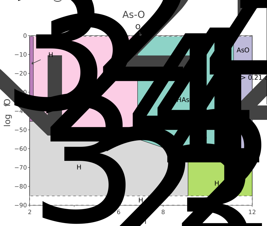
The dominant arsenic species over the plane. The upper band is As(V) – H3AsO4, H2AsO4-, HAsO4-2 and AsO4-3 in sequence as pH rises, the ordinary deprotonation of an acid. The lower band is As(III), H3AsO3 and H2AsO3-. The near-horizontal line between them is the redox boundary, and it is the one that matters: it sits at a fugacity most natural waters straddle, which is why arsenic speciation in groundwater is so often finely balanced.
The two shaded strips are not species. O2(g) > 0.21 atm is above
atmospheric oxygen and H2(g) > 1 atm below the stability of water:
conditions outside them do not occur, and the regions there are drawn only
to show the boundary continuing.
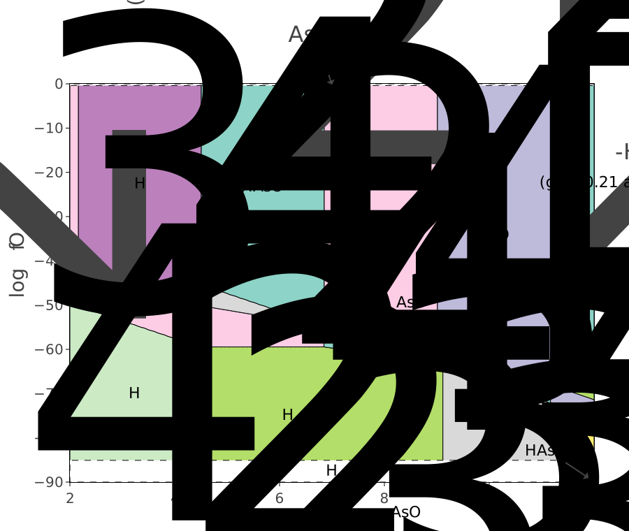
The same plane, now coloured by the second most abundant species. This is the same trace with its target level set to sub-predominant, over the same results – no second simulation was needed.
Two species appear here that are nowhere in the first diagram: H4AsO3+ and HAsO3-2. Neither ever dominates anywhere, so a predominance diagram alone would say they do not exist.
It is also a map of how sharp the first diagram is. Where the sub-dominant species is the neighbour across a boundary, the two are comparable and the boundary is a gradual change; where it is something else entirely, the dominant species holds the field decisively. A predominance diagram draws lines, and the lines are not cliffs – this is the plot that says how steep each one is.
Try it
Narrow the fugacity range to the water stability field and see how much of the diagram is actually reachable.
Change the background electrolyte from NaCl to something arsenic complexes with and watch new regions appear.
Switch the sub-dominant trace back to dominant to confirm the two plots read the same results.
Source
Kinniburgh, D. G. and Cooper, D. M. (2011). PhreePlot: Creating graphical output with PHREEQC. Examples 8 and 9 of the PhreePlot manual are the original of this diagram, including the
Fix_H+construction and the water stability limits. See the PhreePlot website.Parkhurst, D. L. and Appelo, C. A. J. (2013). Description of input and examples for PHREEQC version 3. U.S. Geological Survey Techniques and Methods, book 6, chapter A43.
The thermodynamic data is
wateq4f.dat, distributed with PHREEQC.