01 - Results Visualization
One simulation, shown five different ways. This example is not about the chemistry – it reuses the cation exchange column of 11 - Transport and Cation Exchange – but about what can be done with the results once they exist.
A reactive transport run produces a table with three independent axes: distance along the column, time, and chemical species. No single plot shows all three, so every figure here is a decision about which one to collapse. That choice is the subject.
TITLE Phreeqc Example 11.-- Transport and cation exchange.
SOLUTION 0 CaCl2
units mmol/kgw
temp 25.0
pH 7.0 charge
pe 12.5 O2(g) -0.68
Ca 0.6
Cl @{$ini_conc$}@
SOLUTION 1-40 Initial solution for column
units mmol/kgw
temp 25.0
pH 7.0 charge
pe 12.5 O2(g) -0.68
Na 1.0
K 0.2
N(5) 1.2
END
EXCHANGE 1-40
-equilibrate 1
X 0.0011
END
TRANSPORT
-cells 40
-lengths 0.002
-shifts 100
-time_step 720.0
-flow_direction forward
-boundary_conditions flux flux
-diffusion_coefficient 0.0e-9
-dispersivities @{$dispersivity$}@
-correct_disp true
END
Pick two of three
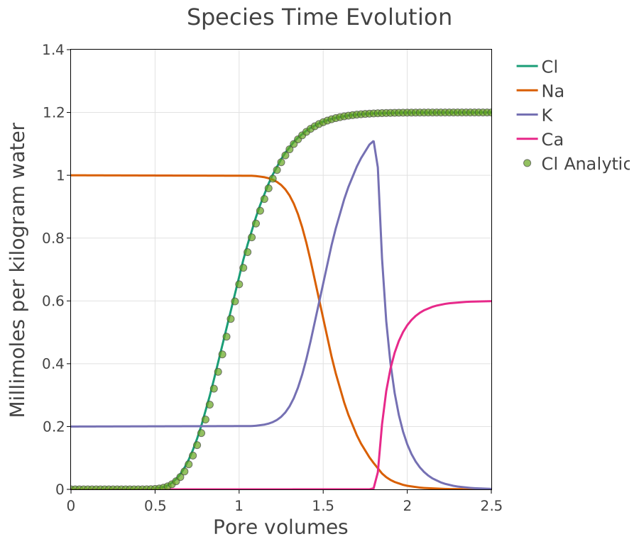
Fix the place, vary time. Concentrations at the boundary cell against pore volumes – the breakthrough curve, and the form in which a column experiment is measured. The analytical chloride is drawn with it as the check described in 11 - Transport and Cation Exchange.
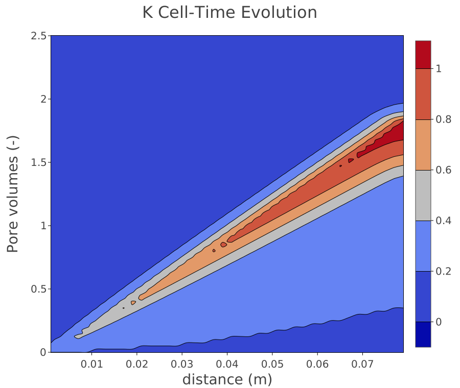
Keep both, drop the species. Potassium over distance and time as a colour map: one species, the whole run. Fronts appear here as diagonal bands, and their slope is a velocity – which is the thing neither a breakthrough curve nor a profile shows directly.
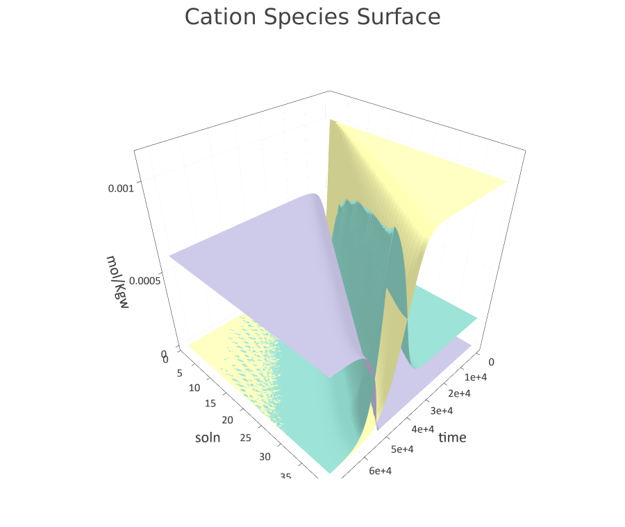
The same, as a surface. Several species at once over the same two axes. Harder to read a value from, easier to see the shape of; useful for finding where something interesting happens before plotting it properly.
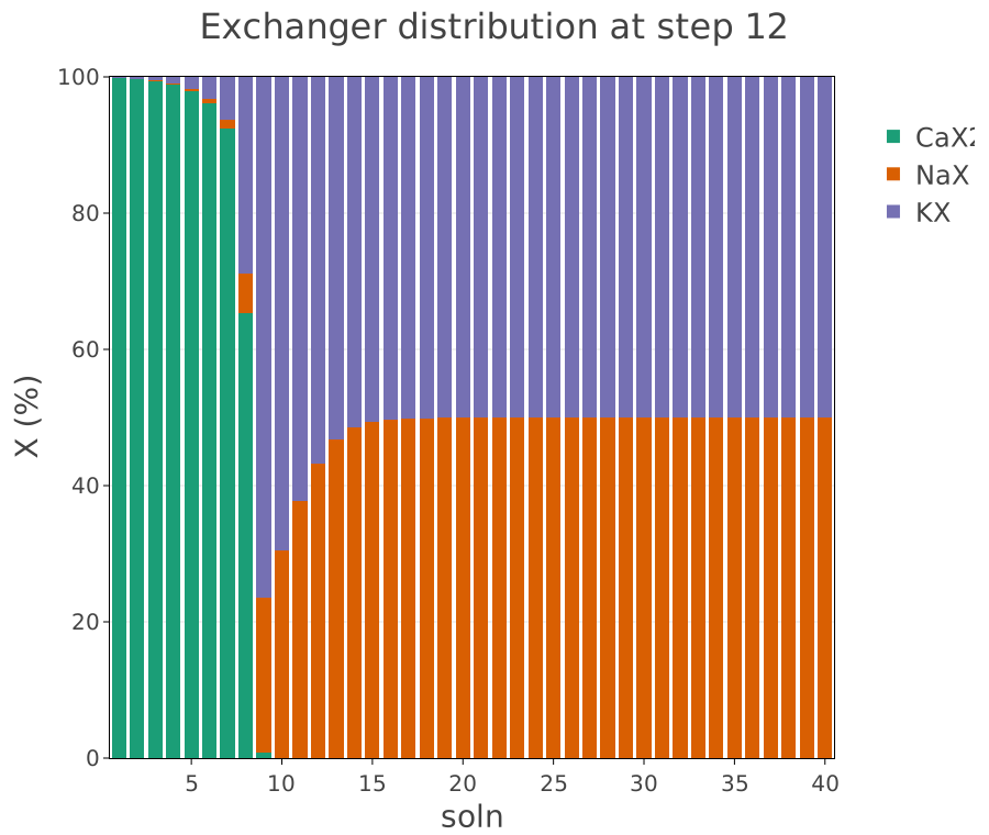
Fix the time, vary the place. The exchanger composition along the column at step 12, as percentages of the sites.
This is the complement of the first figure and the one that explains it. The breakthrough curve shows what came out; this shows what the column is holding, and the replacement of sodium and potassium by calcium moving along as a front is the mechanism behind the effluent curve.
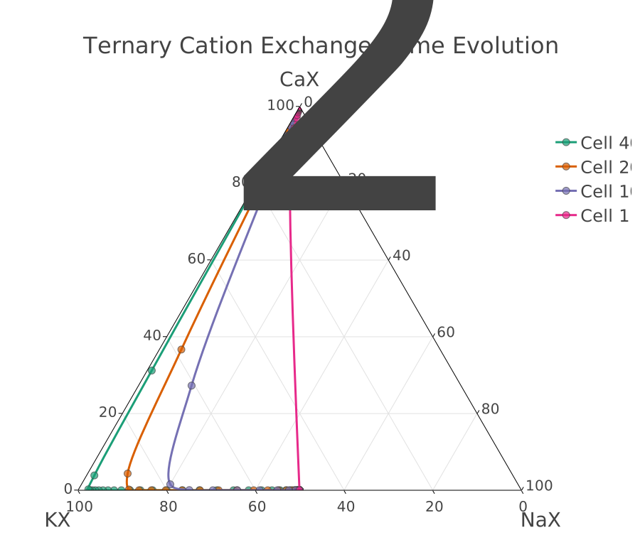
Drop the axes entirely. The three exchangeable cations sum to 100 %, so their composition is two independent numbers and fits on a ternary diagram. Each cell traces a path across it as time passes.
Four cells are drawn – 1, 10, 20 and 40. Their paths lie close to one another, which says that every part of the column passes through essentially the same sequence of exchanger compositions, just at different times. That is a statement about the process rather than about any one location, and none of the four figures above can make it.
The table
Time (sec) |
Cl (mmoles) |
Na (mmoles) |
K (mmoles) |
Ca (mmoles) |
|---|---|---|---|---|
0 |
0 |
1 |
0.2 |
0 |
720 |
0 |
1 |
0.2 |
0 |
1440 |
0 |
1 |
0.2 |
0 |
2160 |
0 |
1 |
0.2 |
0 |
2880 |
0 |
1 |
0.2 |
0 |
3600 |
0 |
1 |
0.2 |
0 |
4320 |
0 |
1 |
0.2 |
0 |
5040 |
0 |
1 |
0.2 |
0 |
5760 |
3.099695935216e-19 |
1 |
0.2 |
0 |
6480 |
1.500905973391e-14 |
1 |
0.2 |
0 |
7200 |
6.3378101301940005e-12 |
1 |
0.2 |
0 |
7920 |
4.494806174889e-10 |
1 |
0.2 |
0 |
8640 |
1.148716182625e-08 |
1 |
0.2 |
0 |
9360 |
1.502206811058e-07 |
1 |
0.2 |
0 |
10080 |
1.22254281191e-06 |
1 |
0.2 |
0 |
10800 |
6.992469583284e-06 |
0.9999999999999001 |
0.2000000000001 |
0 |
11520 |
3.0480434402039997e-05 |
0.9999999999998 |
0.2000000000002 |
0 |
12240 |
0.0001071736884874 |
0.9999999999996 |
0.2000000000004 |
0 |
12960 |
0.0003167880505857 |
0.9999999999990999 |
0.2000000000009 |
0 |
13680 |
0.0008119152403764 |
0.9999999999981001 |
0.2000000000019 |
0 |
14400 |
0.001847753784 |
0.9999999999954999 |
0.2000000000045 |
0 |
15120 |
0.003804229075475 |
0.9999999999815 |
0.2000000000185 |
0 |
15840 |
0.007191769366246 |
0.9999999999194 |
0.20000000008069999 |
0 |
16560 |
0.012635060222689998 |
0.9999999996769 |
0.2000000003232 |
0 |
17280 |
0.020834137170530002 |
0.9999999988263 |
0.2000000011738 |
0 |
18000 |
0.03250742767479 |
0.9999999961114001 |
0.2000000038887 |
0 |
18720 |
0.04832522920503 |
0.9999999881420999 |
0.20000001185779998 |
0 |
19440 |
0.06884373211788 |
0.9999999664316 |
0.20000003356819998 |
0 |
20160 |
0.09444901160173 |
0.9999999111043 |
0.20000008889530002 |
0 |
20880 |
0.1253179893805 |
0.9999997783000001 |
0.20000022169929998 |
0 |
21600 |
0.1614000573129 |
0.9999994762263 |
0.2000005237725 |
0 |
22320 |
0.20241969718269998 |
0.9999988216498 |
0.2000011783484 |
0 |
23040 |
0.24789764663570002 |
0.9999974639168 |
0.20000253607989998 |
0 |
23760 |
0.2971862880203 |
0.9999947567684 |
0.200005243227 |
0 |
24480 |
0.3495140484272 |
0.9999895484264999 |
0.2000104515675 |
0 |
25200 |
0.40403357709590004 |
0.9999798465372999 |
0.2000201534554 |
0 |
25920 |
0.45986908597389997 |
0.9999622949276 |
0.2000377050638 |
0 |
26640 |
0.5161592448412999 |
0.9999313715105 |
0.2000686284796 |
0 |
27360 |
0.5720931802482 |
0.9998781779365 |
0.20012182205239998 |
0 |
28080 |
0.6269382550202 |
0.9997886375294001 |
0.2002113624584 |
0 |
28800 |
0.6800592808307 |
0.9996408433259 |
0.2003591566607 |
0 |
29520 |
0.7309295762311 |
0.9994011963713001 |
0.2005988036142 |
0 |
30240 |
0.7791348087955 |
0.9990188398079001 |
0.2009811601767 |
0 |
30960 |
0.824370867474 |
0.9984177243093 |
0.2015822756744 |
0 |
31680 |
0.8664371340724 |
0.9974854440118 |
0.2025145559711 |
0 |
32400 |
0.9052265038216 |
0.9960577965183 |
0.2039422034634 |
0 |
33120 |
0.9407133877476 |
0.9938979448207 |
0.20610205515990002 |
0 |
33840 |
0.9729407531493001 |
0.9906693148514 |
0.2093306851283 |
0 |
34560 |
1.0020070550459999 |
0.9859023902485 |
0.2140976097306 |
0 |
35280 |
1.028053705196 |
0.9789581360882 |
0.2210418638904 |
0 |
36000 |
1.051253532901 |
0.9689960047788 |
0.2310039951996 |
0 |
36720 |
1.071800523379 |
0.9549633446588 |
0.24503665531950003 |
0 |
37440 |
1.0899009800300001 |
0.9356347669942 |
0.2643652329843 |
0 |
38160 |
1.105766147279 |
0.909738463714 |
0.2902615362648 |
0 |
38880 |
1.1196062494930001 |
0.8761960898604 |
0.323803910119 |
0 |
39600 |
1.131625845338 |
0.8344533299762 |
0.365546670004 |
0 |
40320 |
1.142020362045 |
0.7847919648582 |
0.4152080351229 |
0 |
41040 |
1.150973656035 |
0.7284538370877001 |
0.4715461628945 |
3.527692818409e-25 |
41760 |
1.158656441394 |
0.6674661293038999 |
0.5325338706794 |
4.210831922196e-23 |
42480 |
1.165225432016 |
0.6042301756361 |
0.5957698243484999 |
2.1112644179359998e-21 |
43200 |
1.170823053923 |
0.5410707040733 |
0.6589292959126001 |
9.153155272165e-20 |
43920 |
1.175577598779 |
0.47991770646410004 |
0.7200822935230999 |
3.5143308904239995e-18 |
44640 |
1.179603706072 |
0.42217463625970003 |
0.7778253637289 |
1.2072133357479998e-16 |
45360 |
1.183003078326 |
0.3687296863928 |
0.831270313597 |
3.694071189028e-15 |
46080 |
1.1858653501440002 |
0.3200378092874 |
0.8799621907034 |
1.035721727649e-13 |
46800 |
1.188269047044 |
0.27622844301579996 |
0.9237715569711 |
2.657316513578e-12 |
47520 |
1.190282583742 |
0.23719604397229999 |
0.9628039558955 |
6.272120759453e-11 |
48240 |
1.1919652634100002 |
0.20268026595570002 |
0.9973197312302001 |
1.4041082268950001e-09 |
48960 |
1.193368249524 |
0.1723175378763 |
1.0276824027 |
2.9709432256e-08 |
49680 |
1.194535490349 |
0.14569865254900002 |
1.054300174308 |
5.865691926516e-07 |
50400 |
1.195504582884 |
0.1223834694148 |
1.077593517021 |
1.1506780068630001e-05 |
51120 |
1.19630756853 |
0.1019262302484 |
1.09765724114 |
0.0002082643040654 |
51840 |
1.196971656898 |
0.08381480430459 |
1.109525476356 |
0.0033298596681490002 |
52560 |
1.197519877322 |
0.06668225215375 |
1.024937205368 |
0.05419027123916 |
53280 |
1.197971659937 |
0.05053198361894 |
0.7350507092904 |
0.207208653549 |
54000 |
1.1983433497520002 |
0.03879701353344 |
0.5356918133817 |
0.31275558654860003 |
54720 |
1.1986486582040001 |
0.03007678319726 |
0.40211880019659996 |
0.3839022083108 |
55440 |
1.198899057198 |
0.023444635472219998 |
0.30685223670469997 |
0.4348515639204 |
56160 |
1.199104120993 |
0.01834047970582 |
0.2366187844776 |
0.4725203679181 |
56880 |
1.199271821253 |
0.01438416332256 |
0.1838015686767 |
0.5009071340114001 |
57600 |
1.199408780438 |
0.01130287551729 |
0.1435541335456 |
0.5225714954803 |
58320 |
1.199520488471 |
0.008894854146136 |
0.1125953624841 |
0.5392548916968001 |
59040 |
1.199611487223 |
0.007008145844608 |
0.08861328626373001 |
0.5521892839574001 |
59760 |
1.199685527006 |
0.005526939763041 |
0.06993373970834 |
0.5622696602753 |
60480 |
1.199745698858 |
0.004362237384878 |
0.05532050322144 |
0.5701586297071001 |
61200 |
1.1997945459900001 |
0.0034452316226400003 |
0.043847402190319996 |
0.576353683103 |
61920 |
1.1998341573940001 |
0.002722483621173 |
0.03481279238995 |
0.5812323620030001 |
62640 |
1.199866246232 |
0.0021523437323109997 |
0.02768046310685 |
0.5850835965882 |
63360 |
1.199892215323 |
0.0017022599005469998 |
0.022037745425940003 |
0.5881299973437 |
64080 |
1.199913211686 |
0.001346733077458 |
0.017565220330539998 |
0.590544023302 |
64800 |
1.1999301718820001 |
0.0010657521983839999 |
0.01401446576925 |
0.5924598910212999 |
65520 |
1.199943859609 |
0.0008435890590553 |
0.01119149962915 |
0.5939824556603001 |
66240 |
1.199954896813 |
0.000667865908903 |
0.008944331671829 |
0.5951939012134 |
66960 |
1.1999637893780002 |
0.0005288312741436999 |
0.007153523667664 |
0.5961588225322 |
67680 |
1.1999709483010002 |
0.0004187957410809 |
0.005724978921465999 |
0.5969281126714 |
68400 |
1.199976707113 |
0.0003316912253529 |
0.004584400975147 |
0.5975419539019999 |
69120 |
1.1999813361849998 |
0.0002627259547465 |
0.003673012862258 |
0.5980321305934 |
69840 |
1.199985054462 |
0.0002081138872308 |
0.00294423532525 |
0.5984238253953 |
70560 |
1.199988039067 |
0.0001648621778509 |
0.002361099157963 |
0.5987370193334001 |
71280 |
1.199990433149 |
0.00013060402175539998 |
0.001894222604932 |
0.5989875866877 |
72000 |
1.199992352295 |
0.0001034670377818 |
0.0015202257368670002 |
0.5991881536136 |
Results are also available as a table, which is what to use when a number is wanted rather than a shape.
What it shows
That choosing a plot is choosing a question. The same results support a breakthrough curve, a profile, a map and a composition path, and each discards something the others keep.
Source
Parkhurst, D. L. and Appelo, C. A. J. (2013). Description of input and examples for PHREEQC version 3. U.S. Geological Survey Techniques and Methods, book 6, chapter A43. The model is Example 11 of that manual.
Appelo, C. A. J. and Postma, D. (2005). Geochemistry, Groundwater and Pollution, 2nd edition. Balkema, Leiden.