02 - Mineral Solubility¶

Gypsum (CaSO₄·2H₂O) and anhydrite (CaSO₄) are the same salt, one hydrated and one not, and which of them is stable depends on temperature and pressure. This example computes the solubility of both across that range and compares the result with measurements.

It is the clearest case in this set of a model being tested rather than applied. The answer is known from experiment, so the figures show agreement and disagreement rather than a prediction to be taken on trust.

What is computed¶

Two calculations, in sequence.

First the saturation index of both minerals in a solution in equilibrium with one of them, as temperature varies at 1 atm. Where the two curves cross is the transition: below it gypsum is the stable phase, above it anhydrite.

Then the solubility of each – how much dissolves – as a function of both temperature and pressure, at 1, 500 and 1000 atm.

The results¶

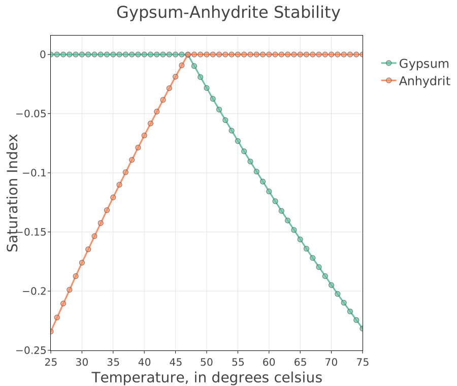
Saturation index of gypsum and anhydrite against temperature, the two curves crossing — Saturation index of the two minerals against temperature at 1 atm. The crossing point is the only part of this figure that matters: on one side of it gypsum is stable and anhydrite would dissolve, on the other the reverse.¶

The transition is around 55-60 °C at atmospheric pressure, which is why gypsum is what you find at the surface and anhydrite what you find at depth in an evaporite sequence.

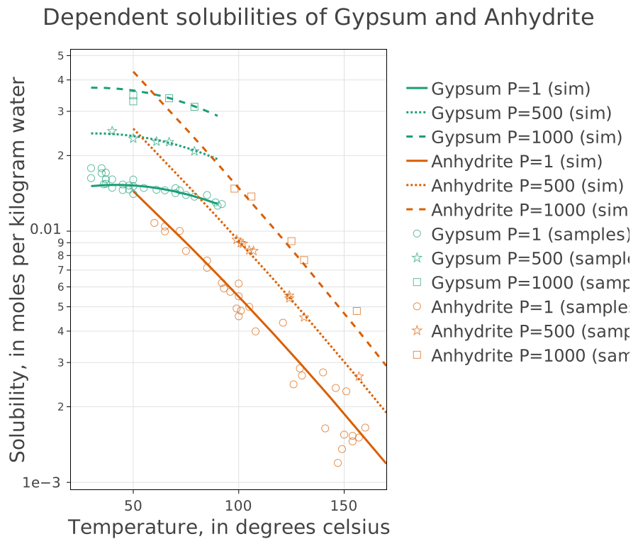
Solubility of gypsum and anhydrite against temperature at three pressures, with measurements — Solubility against temperature at three pressures, with the computed curves and the experimental data on the same axes – six of each, marked `(sim)` and `(samples)`.¶

Two things to read. The **retrograde solubility**: both minerals become *less* soluble as the water warms over much of this range, which is the opposite of most salts and is why warming a calcium sulfate brine makes it precipitate. And the **pressure effect**: raising pressure increases solubility, because dissolution reduces the total volume.

The agreement between curves and points is the result. Where they part company, the thermodynamic data is being extrapolated beyond where it was fitted – which a saturation index will never tell you on its own.

What it shows¶

That a database is a set of fitted constants with a range of validity, and that the way to find that range is to put calculation and measurement on the same axes.

22 - Gas Solubilities does the same for CO₂ at high pressure, where the discrepancy is large enough to need a different equation of state.

Source¶

Parkhurst, D. L. and Appelo, C. A. J. (2013). Description of input and examples for PHREEQC version 3. U.S. Geological Survey Techniques and Methods, book 6, chapter A43. This is Example 2 of that manual, including the experimental solubility data it is compared against.