01 - Monte Carlo Analysis
Every input to a geochemical model is uncertain – the temperature was measured, the pH was measured, the equilibrium constant came from a database with its own error bars. The usual practice is to run the model once with best estimates and report a single number. This example does the other thing: it gives four inputs distributions instead of values, runs the model a thousand times, and looks at the distribution of the answer.
The model is the seawater speciation of the PHREEQC manual’s Example 1, with uranium added. The output of interest is the saturation index of uraninite.
The four uncertain inputs
Input |
Distribution |
Why that shape |
|---|---|---|
Temperature |
Normal, N(25, 1) °C |
A measurement with symmetric error. |
Uraninite log K |
Triangular on [-5, -2], peak -3.5 |
A constant known only as a range with a best guess – which is what
the literature often gives. The peak sits on the -3.49 of
|
pH |
Uniform on [8.1, 8.3) |
A value known to lie in an interval, with no reason to prefer any part of it. |
U concentration |
Lognormal, mean 3.3 ppb, s.d. 0.5 ppb |
A concentration cannot be negative, and lognormal is the usual choice for one. |
The moments given for the lognormal are the concentration’s own mean and standard deviation, not those of its logarithm. The two parameterisations are easy to confuse and give noticeably different distributions.
The seed is 1, so every run of this project draws the same thousand samples and produces the same figures. A seed of 0 would draw new ones each time. Fix the seed while you are developing a model and comparing changes; unfix it when you want to know whether a conclusion depends on the sample.
Running it a thousand times
A Monte Carlo Study wraps the PHREEQC study: it draws a value for each of the four inputs, runs the speciation, records the output, and repeats. The PHREEQC input itself is unchanged – it is the same parameterised input any other study would run.
TITLE Example 1.--Add uranium and speciate seawater.
SOLUTION 1 SEAWATER FROM NORDSTROM AND OTHERS (1979)
units ppm
pH @{$ph_param$}@
pe 8.451
density 1.023
temp @{$temp_param$}@
redox O(0)/O(-2)
Ca 412.3
Mg 1291.8
Na 10768.0
K 399.1
Fe 0.002
Mn 0.0002 pe
Si 4.28
Cl 19353.0
Alkalinity 141.682 as HCO3
S(6) 2712.0
N(5) 0.29 gfw 62.0
N(-3) 0.03 as NH4
U @{$u_ppb$}@ ppb N(5)/N(-3)
O(0) 1.0 O2(g) -0.7
SOLUTION_MASTER_SPECIES
U U+4 0.0 238.0290 238.0290
U(4) U+4 0.0 238.0290
U(5) UO2+ 0.0 238.0290
U(6) UO2+2 0.0 238.0290
SOLUTION_SPECIES
#primary master species for U
#is also secondary master species for U(4)
U+4 = U+4
log_k 0.0
U+4 + 4 H2O = U(OH)4 + 4 H+
log_k -8.538
delta_h 24.760 kcal
U+4 + 5 H2O = U(OH)5- + 5 H+
log_k -13.147
delta_h 27.580 kcal
#secondary master species for U(5)
U+4 + 2 H2O = UO2+ + 4 H+ + e-
log_k -6.432
delta_h 31.130 kcal
#secondary master species for U(6)
U+4 + 2 H2O = UO2+2 + 4 H+ + 2 e-
log_k -9.217
delta_h 34.430 kcal
UO2+2 + H2O = UO2OH+ + H+
log_k -5.782
delta_h 11.015 kcal
2UO2+2 + 2H2O = (UO2)2(OH)2+2 + 2H+
log_k -5.626
delta_h -36.04 kcal
3UO2+2 + 5H2O = (UO2)3(OH)5+ + 5H+
log_k -15.641
delta_h -44.27 kcal
UO2+2 + CO3-2 = UO2CO3
log_k 10.064
delta_h 0.84 kcal
UO2+2 + 2CO3-2 = UO2(CO3)2-2
log_k 16.977
delta_h 3.48 kcal
UO2+2 + 3CO3-2 = UO2(CO3)3-4
log_k 21.397
delta_h -8.78 kcal
PHASES
Uraninite
UO2 + 4 H+ = U+4 + 2 H2O
log_k @{$logK_param$}@
delta_h -18.630 kcal
END
Reading the results
A Univariate Statistics Analysis summarises each input and the output – count, mean, exact median and percentiles, sample variance and standard deviation – and bins them for the histograms. The statistics table gives the same figures per column.
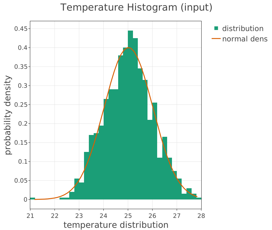
The sampled temperatures, with the normal density of the sample’s own mean and standard deviation drawn over them. This plot is a check on the sampling, not a result: the histogram should follow the curve, and if it does not with a thousand draws, something is wrong before the chemistry is reached.
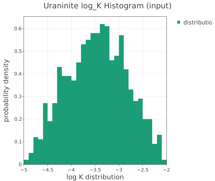
The uraninite log K, triangular on [-5, -2] with its peak at -3.5. The shape is clearly not normal, which matters for what follows.
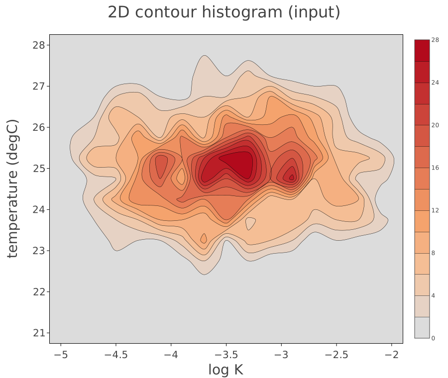
log K against temperature as a two-dimensional histogram. The two were drawn independently, so the density here should be the product of the two marginal shapes and show no trend of one against the other. A tilt in this plot would mean the sampling had introduced a correlation nobody asked for, which is worth checking before interpreting anything downstream.
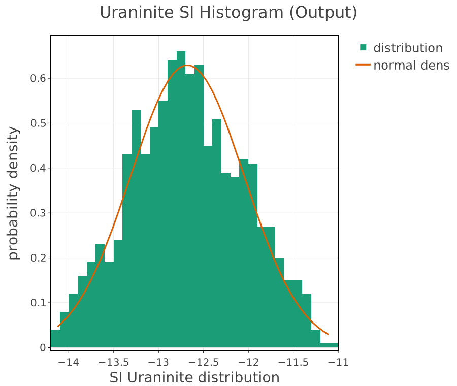
The answer: the saturation index of uraninite across the thousand runs. It is triangular, not normal – it has inherited the shape of the log K distribution almost unchanged. The normal density drawn over it, of the same mean and standard deviation, is there to show how poorly it fits.
This is the result that a single run with best estimates could not have given, and the reason to summarise an uncertain output by more than a mean and a standard deviation: those two numbers describe a bell, and this is not one.
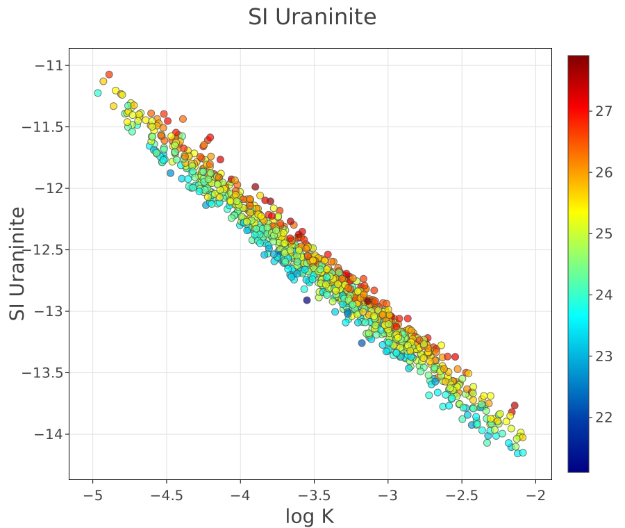
Why. The saturation index against log K, with temperature as the marker colour. The points fall on a line of slope -1, which is not an empirical finding but the definition showing through:
The ion activity product is set by the solution and does not depend on what the database says the mineral’s constant is, so moving log K by one unit moves SI by one unit the other way, exactly.
What the plot actually tells you is the scatter about that line: it is everything the other three inputs contribute together, and it is small. Of the four uncertainties, one dominates the answer.
That is the practical finding, and it is actionable in a way the histogram alone is not: to narrow this prediction, find a better value for the uraninite log K. Measuring the temperature more precisely would be wasted effort.
The statistics table
statistic |
key |
temp_param |
logK_param |
SI Uraninite |
|---|---|---|---|---|
Sum |
sum_v |
25020.526830365365 |
-3465.2934392050333 |
-12679.373161474161 |
Total Count |
count_v |
1000 |
1000 |
1000 |
Mean |
mean_v |
25.020526830365366 |
-3.465293439205033 |
-12.67937316147416 |
Median |
median_v |
25.026808103372513 |
-3.449544106980711 |
-12.69571460039 |
Variance (sample, n - 1) |
variance_v |
0.9924055431501393 |
0.39171917757961355 |
0.4017245169861508 |
Standard deviation (sample) |
std_v |
0.9961955345965667 |
0.6258747299417141 |
0.6338174161271926 |
Minimum |
min_v |
21.101862788293072 |
-4.965630635268282 |
-14.15673151033 |
Maximum |
max_v |
27.907380639448185 |
-2.086382849181004 |
-11.07404083172 |
Percentile 0.05 |
perc_0.05 |
23.389969873562617 |
-4.521451539447734 |
-13.7667662561235 |
Percentile 0.95 |
perc_0.95 |
26.706227598934287 |
-2.4240666453812802 |
-11.6118548313625 |
A caution
The four inputs here are drawn independently, and in geochemistry some inputs are not independent. pH and the partial pressure of CO2 are the obvious pair: sampled separately, they will combine into waters that cannot exist, and the model will dutifully speciate them. The resulting distribution is then wider than reality and wrong in shape.
Choose which inputs to randomise with that in mind, and where two are coupled, either sample one and derive the other or sample them jointly.
Source
Parkhurst, D. L. and Appelo, C. A. J. (2013). Description of input and examples for PHREEQC version 3. U.S. Geological Survey Techniques and Methods, book 6, chapter A43. The seawater composition is Example 1 of that manual; the uranium and its uncertainty were added here.