01 - Fit Kinetics
The first fit in this set with a chemical model behind it: the rate constant for quartz dissolution, fitted to dissolved silicon measured over five years.
It is PhreePlot’s quartz kinetics example. Everything from 01 - Analytic Function Fitting carries over – a residual expression, fitting parameters with bounds, Ceres underneath – and one thing is new, which is how the measurements are matched to the simulation.
The model
# Kinetics of quartz dissolution
# from Appelo 'Get-going sheet #11'
#TRANSPORT
# -initial_time 0
RATES
#1 dQu/dt = -k * (1 - SR(Quartz). k = 10^-13.7 mol/m2/s (25 C)
#2 parm(1) = A (m2), parm(2) = V (dm3) recalculate to mol/dm3/s
Quartz # rate name
-start
10 moles = parm(1) / parm(2) * (m/m0)^0.67 * 10^@{$log_k$}@ * (1 - SR("Quartz"))
20 save moles * time # integrate. save and time must be in rate definition
-end # moles count positive when added to solution
KINETICS # Sediment: 100% qu, grain size 0.1 mm, por 0.3, rho_qu 2.65 kg/dm3
Quartz # rate name
-formula SiO2
-m0 102.7 # initial moles of quartz
-parms 22.7 0.162 # parameters for rate eqn. Here:
# Quartz surface area (m2/kg sediment), water filled porosity (dm3/kg sediment)
-steps 1.5768e8 in 100 steps # 1.5768e8 seconds = 5 years
-tol 1e-8 # integration tolerance, default 1e-8 mol
INCREMENTAL_REACTIONS false # start integration from previous step
SOLUTION 1
END
A RATES block gives the dissolution rate of quartz, with the constant as
the fitting parameter:
10 moles = parm(1) / parm(2) * (m/m0)^0.67 * 10^@{$log_k$}@ * (1 - SR("Quartz"))
Three things are happening in that line. The rate is proportional to surface
area per litre of water, parm(1)/parm(2); it shrinks as the grains do,
through (m/m0)^0.67 – the two-thirds power of a volume being an area;
and it stops at equilibrium, through 1 - SR("Quartz"), which goes to zero
as the saturation ratio reaches one.
Only log_k is fitted. The geometry is measured: a sediment of pure quartz
at 0.1 mm grain size, 22.7 m² of surface per kg and 0.162 l of water per kg.
The KINETICS block integrates this over 1.5768×10⁸ seconds – five years
– in 100 steps.
Matching observations to steps
The data is 50 rows and the simulation is 100 steps, and the measurements are not evenly spaced. So each observation names the step it belongs to:
targetSimulationStep   secTime   time    Si_calc   SIQtz   error   Si_obs
1                      1576800   0.05    0.0045    -1.3678 -0.0015 0.003
5                      7884000   0.25    0.0206    -0.706   0.0023 0.0229
6                      9460800   0.3     0.0242    -0.6359  0.0005 0.0247
This is vector mode, and it is the difference from 01 - Analytic Function Fitting. There, each data row was an independent simulation: 67 rows meant 67 evaluations of the model. Here all 50 observations come from one simulation, and each is joined to the row of the step it names.
The distinction is not a detail of bookkeeping. A kinetic run is a single trajectory – step 50 depends on every step before it – so the 50 measurements are not 50 independent experiments and cannot be simulated as such. Vector mode is what makes a time series fittable at all, and it costs one simulation per iteration instead of fifty.
The residual is
#Si_observed# - #Si#*1000
with the factor of 1000 converting PHREEQC’s mol/kgw to the mmol/kgw the observations are in. Unit conversions live in the residual, where they are visible, rather than in the data file.
log_k starts at -13 and is bounded to ±100. The published rate constant
for quartz is around 10⁻¹³·⁷ mol/m²/s at 25 °C, so the starting value is
roughly right – and for a model this non-linear, starting roughly right is
not optional.
The result
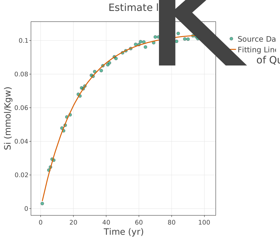
Silicon against time, measurements and fitted model. The curve has the
shape kinetics gives it: steep at first, where the water is far from
saturation and 1 - SR is near one, then flattening as the solution
approaches equilibrium with quartz and the driving force disappears.
The fit is to the whole trajectory, not to any one point. That is the value of the approach – the early slope constrains the rate constant and the plateau constrains the solubility, and a single constant has to satisfy both at once.
Try it
Start
log_kat -10 and see whether the fit still finds its way back.Halve the surface area in
-parmsand watch the fittedlog_kcompensate – the two are not separable from this data alone.Shorten the run to one year and see what the plateau’s absence does to the standard error.
Source
Kinniburgh, D. G. and Cooper, D. M. (2011). PhreePlot: Creating graphical output with PHREEQC. This is PhreePlot’s quartz kinetics fit. See the PhreePlot website.
Appelo, C. A. J. Get-going sheet #11, cited in the input itself, is the origin of the rate expression and the sediment parameters.
The thermodynamic data is
wateq4f.dat, distributed with PHREEQC (Parkhurst and Appelo, 2013).