01 - Function Surface Drawing

No chemistry at all: the surface \(f(x,y) = -x^2 - y^2\) over the square \([-1, 1] \times [-1, 1]\). The point is the machinery around it. Every model in GibbsStudio is driven the same way – a model that computes something, parametric studies that run it over a range of inputs, and plots that read the single table of results they leave behind – and here that machinery is visible on its own, with an answer you already know.

Start here if you have not built a project before. 02 - Trigonometric Function Drawing continues with the same ideas on a one-dimensional function.

The function

The Function Model holds one expression, named f_out:

f_out = -x*x + -y*y

x and y are project parameters. They have values of their own – both start at 1 – so the model is complete and computable before any study touches it. That matters: a model you cannot run on its own is a model you cannot debug. A Function Study, xyFunction, runs it once and produces a single row.

The project also carries two parameters the function never uses, and they are there to show what a parameter can be:

stringParam    = 'myStringValue'
nameParamEval  = 5*(stringParam == 'myStringValue')

Parameters are not only numbers. stringParam is text, and nameParamEval compares it and does arithmetic on the result – a comparison evaluates to 1 or 0, so this one is 5. Switches built this way turn a condition somewhere in a project into a number an expression can use.

Sweeping two of them

A Parametric Study takes a study and runs it again for every value of a parameter. xParameterRange targets xyFunction and sweeps:

x = range(-1, 1, 0.2)

That alone gives a line of results. The second study, yParameterRange, does not target the function study – it targets xParameterRange:

y = range(-1, 1, 0.2)

So the whole x sweep is repeated for each value of y, and the result is the full grid. This is the idea worth taking away from the example: parametric studies chain, and chaining them is how a project gets more than one dimension. Nothing in the function model knows it is being run on a grid.

The results of the chain are one table, with a column for each parameter and each function output. The three plots below all read that same table.

Three views of one result

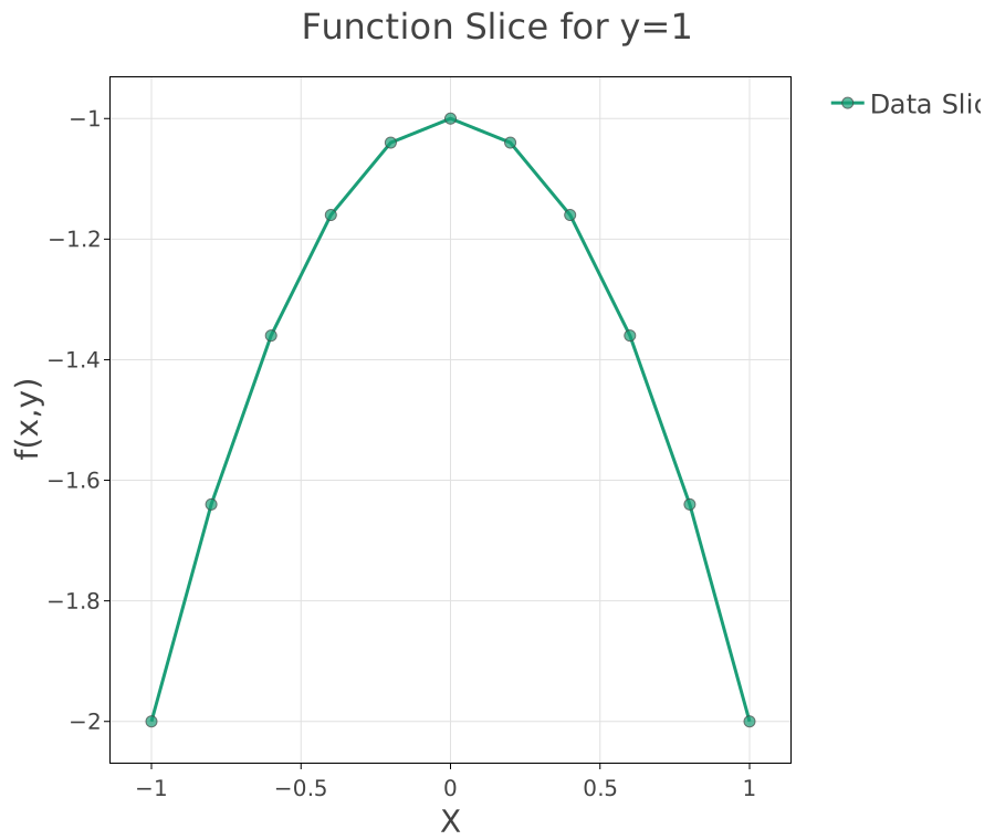
A single slice. The plot reads the grid but shows one line of it, because its data has a local selection on y with the value 1. The title is not fixed text – it is the expression Function Slice for y=#y#, so it reports which slice is on screen. Change the selection and the title follows.

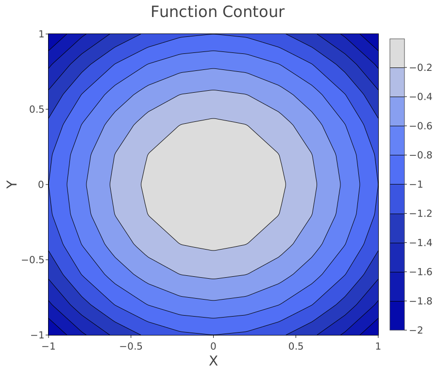
The same table as a contour. The trace is given x and y for position and #f_out# for height, and interpolates linearly between the grid points. Concentric rings centred on the origin, closing in towards the maximum at \(f(0,0) = 0\).

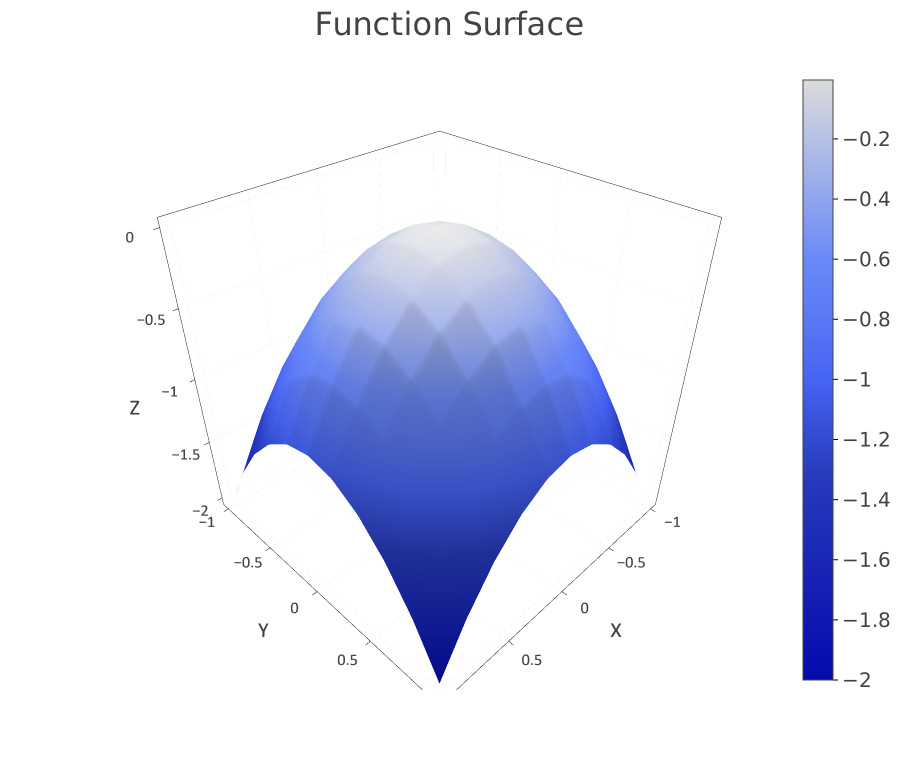
And as a surface, which is what \(-x^2-y^2\) looks like: a dome with its peak at the origin, falling away to \(-2\) at the corners.

Each plot is an independent object reading the same results. None of them re-runs the model, and deleting one does not affect the others.

Try it

• Change the step in either range to 0.1. Nothing else needs editing: the studies produce a finer grid and all three plots redraw from it.

• Change the slice plot’s local selection value from 1 to 0 and watch the title change with it.

• Edit f_out – try -x*x - y*y + 0.5*x*y – and recompute. The plots know nothing about the expression, so they simply show the new surface.