02 - Mineral solubility

A predominance diagram is usually read as a map of regions. This example uses one as a background: it computes the calcite saturation field over pH and calcium, then plots eleven real samples on top of it, so that each sample can be read off against the boundary between dissolving and precipitating.

It is also the second example of running a table of samples through PHREEQC one row at a time – the Water Chemistry set has the other – and the two are worth comparing, because they use the mechanism for different ends.

The samples

analysis_data.tsv

name	Ca	K	Na	pH
Well1	3.00E-01	3.10E+00	1.10E+00	5.00E+00
Well2	4.00E-01	1.10E-01	1.20E+00	4.50E+00
Well3	8.00E-01	3.10E-01	1.50E+00	5.00E+00
Well4	9.00E-01	1.40E-01	1.90E+00	6.54E+00
Well5	1.20E+00	3.60E+00	2.20E+00	4.20E+00
Well6	2.00E-01	2.30E+00	1.23E+00	7.60E+00
River1	1.00E+00	1.21E+00	3.20E+00	4.20E+00
River2	1.00E-01	2.30E-01	1.23E-01	7.00E+00
Well6	2.20E+00	1.60E+00	2.18E+00	4.12E+00
River3	2.00E-01	5.30E-01	1.23E-01	7.10E+00
River4	4.00E-01	2.30E-01	6.66E-01	6.30E+00

Eleven wells, each with calcium, potassium, sodium and pH. These are the columns the input takes; everything else about the water is held fixed.

The parameterised input

SOLUTION 1

   pH        @{$pH_param$}@

   units     mol/kgw

   Fe(3)     1e-2

   Na        @{$Na_param$}@

   Ca        @{$Ca_param$}@

   K         @{$K_param$}@

   Cl        1e-1 charge

   C         1 CO2(g) -3.5

END

Four values come from the table – pH_param, Na_param, Ca_param and K_param. The rest of the solution is fixed: ferric iron at 10 mmol/l, chloride balancing the charge, and carbon in equilibrium with CO2 at a log fugacity of -3.5, which is roughly atmospheric.

That last line is the modelling decision worth noticing:

C         1 CO2(g) -3.5

The carbon is not taken from the analysis. It is set by equilibrium with the atmosphere, which is an assumption about where these samples have been – reasonable for a water that has been exposed to air, wrong for a confined aquifer or a sample that has degassed since collection. Every point in the figures below inherits it.

A Discrete Data Study then runs the input once per row of the table.

The three views

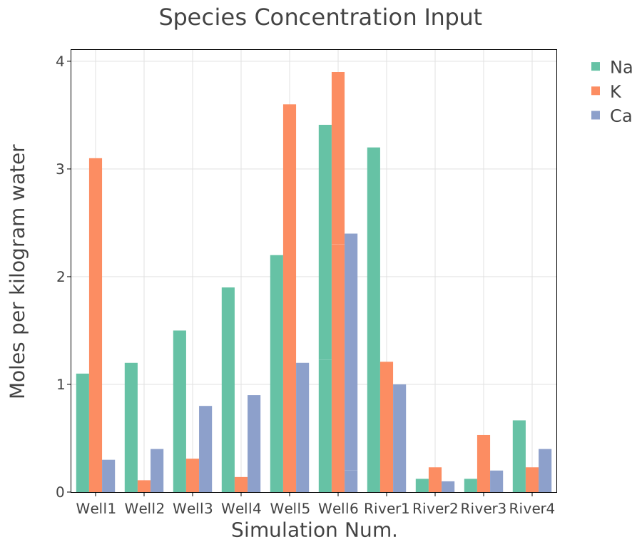
What went in: the three cation concentrations against the simulation number, one point per sample. This is a check rather than a result, and worth running first on any table-driven study – an outlier here is a transcription error or a unit mistake, and it is far cheaper to see it in this plot than to find it later in the chemistry.

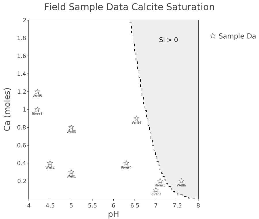
The result. The plane is divided into SI < 0, where a water would dissolve calcite, and SI > 0, where it would precipitate; the eleven samples are drawn on top as points.

The regions come from a predominance study over pH and calcium and the points from the sample runs – two different studies, one pair of axes. The field says what would happen to a water of a given pH and calcium content; the points say where these particular waters sit in relation to that boundary, and how far from it. A sample close to the line is near equilibrium and could move either way with a small change in pH; one deep in the undersaturated field is aggressive towards carbonate.

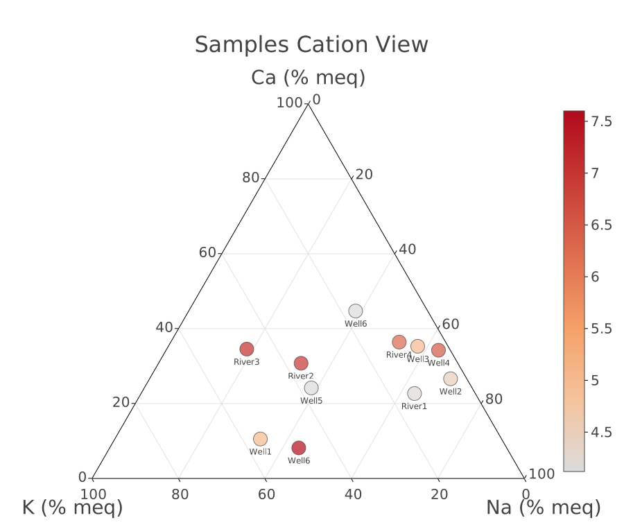
The cation composition of the same samples, as a summary of what distinguishes them.

Try it

• Replace the fixed CO2 fugacity with a measured alkalinity column and compare where the points land.

• Add your own table with the same column names: nothing in the project refers to these particular wells.

• Switch the background field to dolomite or gypsum saturation and plot the same samples against it.

Source

• Parkhurst, D. L. and Appelo, C. A. J. (2013). Description of input and examples for PHREEQC version 3. U.S. Geological Survey Techniques and Methods, book 6, chapter A43.

The sample data is synthetic.