06 - Reaction Path Calculations
Pure water attacking K-feldspar, and the sequence of clay minerals that forms as it does. This is the classic reaction path of low-temperature geochemistry, and the example computes it three different ways to show they agree.
The chemistry is incongruent dissolution: K-feldspar does not simply dissolve into its components. As it breaks down, the aluminium and silicon it releases immediately form something else, and which something depends on how far the reaction has gone. Only the four phases of the original treatment – K-feldspar, gibbsite, kaolinite and K-mica – are considered.
The activity diagram
TITLE Simulation 6A.--React to phase boundaries.
SOLUTION 1 PURE WATER
pH 7.0 charge
temp 25.0
PHASES
Gibbsite
Al(OH)3 + 3 H+ = Al+3 + 3 H2O
log_k 8.049
delta_h -22.792 kcal
Kaolinite
Al2Si2O5(OH)4 + 6 H+ = H2O + 2 H4SiO4 + 2 Al+3
log_k 5.708
delta_h -35.306 kcal
K-mica
KAl3Si3O10(OH)2 + 10 H+ = 3 Al+3 + 3 H4SiO4 + K+
log_k 12.970
delta_h -59.377 kcal
K-feldspar
KAlSi3O8 + 4 H2O + 4 H+ = Al+3 + 3 H4SiO4 + K+
log_k 0.875
delta_h -12.467 kcal
END
TITLE Simulation 6A1.--Find amount of K-feldspar dissolved to
reach gibbsite saturation.
USE solution 1
EQUILIBRIUM_PHASES 1
Gibbsite 0.0 KAlSi3O8 10.0
Kaolinite 0.0 0.0
K-mica 0.0 0.0
K-feldspar 0.0 0.0
END
TITLE Simulation 6A2.--Find amount of K-feldspar dissolved to
reach kaolinite saturation.
USE solution 1
EQUILIBRIUM_PHASES 1
Gibbsite 0.0 0.0
Kaolinite 0.0 KAlSi3O8 10.0
K-mica 0.0 0.0
K-feldspar 0.0 0.0
END
TITLE Simulation 6A3.--Find amount of K-feldspar dissolved to
reach K-mica saturation.
USE solution 1
EQUILIBRIUM_PHASES 1
Gibbsite 0.0 0.0
Kaolinite 0.0 0.0
K-mica 0.0 KAlSi3O8 10.0
K-feldspar 0.0 0.0
END
TITLE Simulation 6A4.--Find amount of K-feldspar dissolved to
reach K-feldspar saturation.
USE solution 1
EQUILIBRIUM_PHASES 1
Gibbsite 0.0 0.0
Kaolinite 0.0 0.0
K-mica 0.0 0.0
K-feldspar 0.0 KAlSi3O8 10.0
END
TITLE Simulation 6A5.--Find point with kaolinite present,
but no gibbsite.
USE solution 1
EQUILIBRIUM_PHASES 1
Gibbsite 0.0 KAlSi3O8 10.0
Kaolinite 0.0 1.0
END
TITLE Simulation 6A6.--Find point with K-mica present,
but no kaolinite
USE solution 1
EQUILIBRIUM_PHASES 1
Kaolinite 0.0 KAlSi3O8 10.0
K-mica 0.0 1.0
END
TITLE Simulation 6B.--Path between phase boundaries.
USE solution 1
EQUILIBRIUM_PHASES 1
Kaolinite 0.0 0.0
Gibbsite 0.0 0.0
K-mica 0.0 0.0
K-feldspar 0.0 0.0
REACTION 1
K-feldspar 1.0
0.04 0.08 0.16 0.32 0.64 1.0 2.0 4.0
8.0 16.0 32.0 64.0 100 200 umol
END
TITLE Simulation 6C.--kinetic calculation
SOLUTION 1
-units mol/kgw
Al 1.e-13
K 1.e-13
Si 3.e-13
EQUILIBRIUM_PHASES 1
Gibbsite 0.0 0.0
Kaolinite 0.0 0.0
K-mica 0.0 0.0
KINETICS 1
K-feldspar
# k0 * A/V = 1e-16 mol/cm2/s * (10% fsp, 0.1mm cubes) 136/cm = 136.e-13 mol/dm3/s
-parms 1.36e-11
-m0 2.16
-m 1.94
-step_divide 1e-6
-steps 1e2 1e3 1e4 1e5 1e6 1e7 1e8
# -steps 1e2 1e3 1e4 1e5 63240.0 64950.0 1347610.0 1010300.0 45242800.0
INCREMENTAL_REACTIONS true
RATES
K-feldspar
-start
10 REM store the initial amount of K-feldspar
20 IF EXISTS(1) = 0 THEN PUT(M, 1)
30 REM calculate moles of reaction
40 SR_kfld = SR("K-feldspar")
50 moles = PARM(1) * (M/M0)^0.67 * (1 - SR_kfld) * TIME
60 REM The following is for printout of phase transitions
80 REM Start Gibbsite
90 if ABS(SI("Gibbsite")) > 1e-3 THEN GOTO 150
100 i = 2
110 GOSUB 1500
150 REM Start Gibbsite -> Kaolinite
160 if ABS(SI("Kaolinite")) > 1e-3 THEN GOTO 200
170 i = 3
180 GOSUB 1500
200 REM End Gibbsite -> Kaolinite
210 if ABS(SI("Kaolinite")) > 1e-3 OR EQUI("Gibbsite") > 0 THEN GOTO 250
220 i = 4
230 GOSUB 1500
250 REM Start Kaolinite -> K-mica
260 if ABS(SI("K-mica")) > 1e-3 THEN GOTO 300
270 i = 5
280 GOSUB 1500
300 REM End Kaolinite -> K-mica
310 if ABS(SI("K-mica")) > 1e-3 OR EQUI("Kaolinite") > 0 THEN GOTO 350
320 i = 6
330 GOSUB 1500
350 REM Start K-mica -> K-feldspar
360 if ABS(SI("K-feldspar")) > 1e-3 THEN GOTO 1000
370 i = 7
380 GOSUB 1500
1000 SAVE moles
1010 END
1500 REM subroutine to store data
1510 if GET(i) >= M THEN RETURN
1520 PUT(M, i)
1530 PUT(TOTAL_TIME, i, 1)
1540 PUT(LA("K+")-LA("H+"), i, 2)
1550 PUT(LA("H4SiO4"), i, 3)
1560 RETURN
-end
USER_PRINT
10 DATA "A: Gibbsite ", "B: Gibbsite -> Kaolinite ", \
"C: Gibbsite -> Kaolinite ", "D: Kaolinite -> K-mica ", \
"E: Kaolinite -> K-mica ", "F: K-mica -> K-feldspar"
20 PRINT \
" Transition Time K-feldspar LA(K/H) LA(H4SiO4)"
30 PRINT " transfer"
40 PRINT " (umoles)"
50 FOR i = 2 TO 7
60 READ s$
70 IF EXISTS(i) THEN PRINT s$, GET(i,1), (GET(1) - GET(i))*1e6, GET(i,2), GET(i,3)
80 NEXT i
END
PRINT; -user_print false
# --Plot the phase boundaries with USER_GRAPH..
PHASES
K_H; KH = K+ - H+; -no_check
SOLUTION 1
pH 11; K 1 K_H 8; Al 1 Gibbsite; Si 1 K-mica
SOLUTION 2
pH 7; K 1 K-mica; Al 1 Gibbsite; Si 1 Kaolinite
SOLUTION 3
pH 7; K 1 K-mica; Al 1 K-feldspar; Si 1 Kaolinite
SOLUTION 4
pH 7; K 1 K_H -1; Al 1 Kaolinite; Si 1 K-feldspar
END
SOLUTION 1
pH 11; K 1 K_H 8; Al 1 K-feldspar; Si 1 K-mica
SOLUTION 2
pH 7; K 1 K-mica; Al 1 K-feldspar; Si 1 Kaolinite
SOLUTION 3
pH 7; K 1 K-mica; Al 1 Gibbsite; Si 1 Kaolinite
SOLUTION 4
pH 7; K 1 K_H -1; Al 1 Gibbsite; Si 1 Kaolinite
END
The input defines the four phases explicitly rather than relying on the database, so that the calculation reproduces the published one exactly.
The path is drawn on axes of log[H₄SiO₄] against log([H⁺][K⁺]) – the two quantities the stability of these phases depends on. The phase boundaries are straight lines on these axes, because each is a reaction with fixed stoichiometry, and that is the whole reason this particular pair of axes is used.
Three ways to the same path
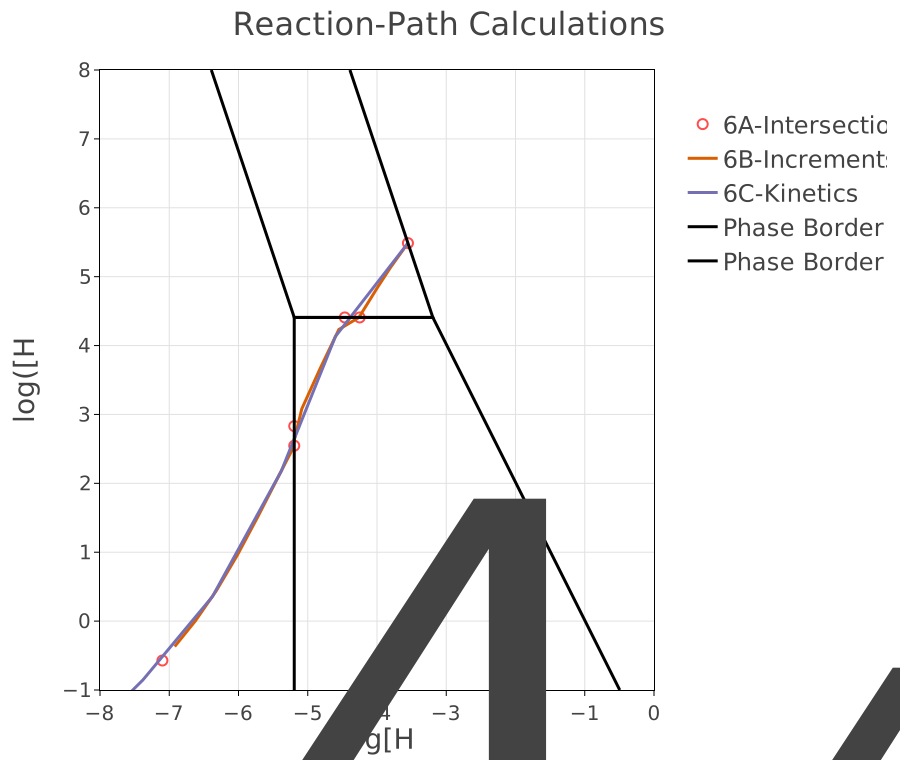
The path, with the phase boundaries drawn over it. It starts at the bottom left in pure water and climbs as feldspar dissolves, crossing from the gibbsite field into kaolinite and on towards K-mica.
The corners are the interesting part. Each is where the path meets a phase boundary, and at that point the mineral that was precipitating begins to redissolve while the next one takes over. The path then runs along the boundary for a while – both phases present, the system buffered – before leaving it.
Three methods are drawn, and they lie on top of each other:
6A, intersections – solve directly for the composition at each phase boundary. Exact, and it gives the corners and nothing between them.
6B, increments – dissolve a fixed amount of feldspar at a time and see where the water goes. Fills in the path, with a resolution set by the step.
6C, kinetics – dissolve feldspar at a rate, so the path is parameterised by time rather than by extent.
Three formulations of the same problem agreeing is the result. 6A says where the corners are, 6B says what the path looks like, and 6C says how long it takes – and the first two cannot answer that last question at all.
What it shows
That a reaction path is a trajectory through a stability diagram, and that the choice of how to compute it is separate from the chemistry. Choose the formulation by what you need to know.
Source
Parkhurst, D. L. and Appelo, C. A. J. (2013). Description of input and examples for PHREEQC version 3. U.S. Geological Survey Techniques and Methods, book 6, chapter A43. This is Example 6 of that manual.
Helgeson, H. C., Garrels, R. M. and Mackenzie, F. T. (1969). Evaluation of irreversible reactions in geochemical processes involving minerals and aqueous solutions – II. Applications. Geochimica et Cosmochimica Acta 33, 455-481. The four phases and the original treatment of this path are theirs.