02 - Fit Langmuir Isotherm¶

Two parameters this time, fitted to a sorption isotherm: zinc on hydrous ferric oxide at fixed pH, over a range of zinc concentrations. The two are the number of sites available and the strength with which zinc binds to them.

It is PhreePlot’s Langmuir isotherm example, and it is the first case here where the parameters are not independent of each other.

A Langmuir model in two lines¶

PHASES

Fix_H+

  H+ = H+

  log_k 0.0

SURFACE_MASTER_SPECIES

  Surf Surf

SURFACE_SPECIES

  Surf = Surf

  log_k  0.0

  Surf + Zn+2 = SurfZn+2                                             # Langmuir model

  log_K @{$log_k$}@                                                      # this is where log_k (updated parameter value) is substituted

PRINT

    -reset false

SOLUTION 1

  -pH @{$pHobs$}@

  -units mmol/L

  Na   1000                                                          # 1 M NaNO3 background electrolyte

  N(5) 1000

  Zn   @{$Znconcn$}@                                                     # <Znconcn> from iso.dat

SURFACE

  Surf @{$M_param$}@                                                          # this is where the max number of sites (updated parameter) is substituted

  -equil 1

  -no_edl

EQUILIBRIUM_PHASES

  Fix_H+ @{$-pHobs$}@  NaOH                                              # pHobs from the fit data file

  -force_equality true

END

The surface is declared from scratch rather than taken from a database:

SURFACE_MASTER_SPECIES
  Surf Surf
SURFACE_SPECIES
  Surf = Surf
  log_k  0.0
  Surf + Zn+2 = SurfZn+2
  log_K @{$log_k$}@

One site type, one reaction, one constant. That is the Langmuir model – a fixed number of identical, independent sites, each either empty or holding one ion – written as chemistry rather than as the usual algebraic isotherm. The familiar hyperbola is a consequence of it, not an input to it.

-no_edl turns off the electrical double layer, which keeps it a pure Langmuir model: with a charged surface the sorption would depend on the accumulated charge as well as on the binding constant, and the two parameters would no longer mean what the model says they mean.

The two fitted parameters are:

M_param, the total number of sites on the surface;
log_k, the binding constant of Surf + Zn+2 = SurfZn+2.

Each data row gives a zinc concentration and a pH, the pH being imposed with the usual Fix_H+ construction. The background is 1 M NaNO3.

Output that GibbsStudio owns¶

The original PhreePlot input carried a USER_PUNCH block to report the sorbed zinc. That block is not used here. GibbsStudio manages SELECTED_OUTPUT and USER_PUNCH itself – they are stripped from any imported input – and the same quantity is requested through a Selected Output object with a punch expression:

SURF("Zn","Surf")

The reason is that these become named columns the rest of the project can refer to. sorbed_Zn_computed is then available to the residual, to the plots and to any view, instead of being a column in a text file that something has to parse.

The residual is measured minus modelled, as always:

#Znsorbed# - #sorbed_Zn_computed#

Eleven data rows, eleven residuals, two unknowns.

The result¶

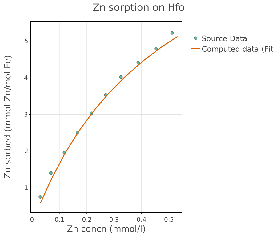
Zinc sorbed against zinc in solution, measurements and fitted Langmuir isotherm — Zinc sorbed against zinc remaining in solution: the isotherm. It rises steeply at low concentration, where sites are plentiful and every added zinc finds one, and bends towards a plateau as the sites fill.¶

Both fitted parameters are visible in that shape, and this is the figure to look at when deciding whether a fit like this is trustworthy. The **plateau** fixes the site density: it is where the surface runs out. The **initial slope** fixes the binding constant. An isotherm measured only on the steep part determines neither separately – many combinations of a larger capacity and a weaker constant give the same early curve – and the fit will still converge and report numbers.

Check the standard errors in the fit output, and check that the data reaches the bend.

Try it¶

Fit only the first four points and compare the standard errors with the full fit.
Turn the double layer back on by removing -no_edl and see how much the fitted constant moves.
Add a second site type and watch the fit improve for reasons that have nothing to do with the chemistry being better described.

Source¶

Kinniburgh, D. G. and Cooper, D. M. (2011). PhreePlot: Creating graphical output with PHREEQC. This is PhreePlot’s Langmuir isotherm fit. See the PhreePlot website.
Langmuir, I. (1918). The adsorption of gases on plane surfaces of glass, mica and platinum. Journal of the American Chemical Society 40, 1361-1403.
The thermodynamic data is wateq4f.dat, distributed with PHREEQC (Parkhurst and Appelo, 2013).